Homework 01
Meet the toolkit and your Data Science Profile
The goal of this assignment is to introduce you to R, RStudio, Git, and GitHub, which you’ll be using throughout the course both to learn the data science concepts discussed in the course and to analyze real data and come to informed conclusions.
1 Getting started
1.1 Prerequisites
First, you need to achieve the following
- Review the Lecture of Week 1
- Read Happy Git with R: Why Git? Why GitHub? (It is OK do a fast read only. You may reconsider later.)
- You have a GitHub account to become a member of the GitHub organization. If you do not have an account follow the instructions on the front page of https://github.com/CU-F23-MDSSB-01-Concepts-Tools.
- You have provided your GitHub username in this form https://forms.office.com/e/fraU0w0gQq (If you provided your name wrongly, write an email to the instructor.)
- Software installations on your computer:
- Read Happy Git with R: Install or upgrade R and RStudio
Follow the instructions to install R and RStudio - Read Happy Git with R: Install Git
Follow the instructions (choose the highly recommended) to install Git SCM (= Source Control Managment) - Install quarto CLI (= Command Line Interface) https://quarto.org/docs/get-started/.
Note: In the following you will do similar things as described in Tutorial: Hello, Quarto and the following two tutorials.
- Read Happy Git with R: Install or upgrade R and RStudio
- In R, install some packages from the following list. You can use the command
install.packages("tidyverse","gitcreds","usethis")
Notes: tidyverse is a collection of many packages it can take some time to install. usethis an gitcreds provide convenient functions to tell your git-installation your GitHub-credentials to push your work back to github via a Personal Access Token (PAT). Read Happy Git with R: Personal access token for HTTPS for how PATs are used similar but not identical to passwords.
Soon, we will need more software: python using the IDE (integrated development environment) Visual Studio Code.
1.2 Terminology
We’ve already thrown around a few new terms, so let’s define them before we proceed.
R and python: Names of the programming language we will be using throughout the course.
RStudio: An integrated development environment developed for R. In other words, a convenient interface for writing and running code.
Git: A version control system.
GitHub: A web platform for hosting version controlled files and facilitating collaboration among users.
quarto: A command line tool which can render (among other things) qmd-files (with text and code chunks) to nice looking html
Repository: A Git repository contains all of your project’s files and stores each file’s revision history.
It’s common to refer to a repository as a repo.
- In this course, assignment you work on will be contained in a personalized git repo.
- For individual assignments, only you will have access to the repo. For team assignments, all team members will have access to a single repo where they work collaboratively.
- All repos associated with this course are housed in the GitHub organization https://github.com/CU-F23-MDSSB-01-Concepts-Tools. The organization is set up such that students can only see repos they have access to, but the course instructors can see all of them.
1.3 Starting slowly step by step
As the course progresses, you are encouraged to explore beyond what the assignments dictate; a willingness to experiment will make you a much better programmer! Before we get to that stage, however, you need to build some basic fluency in the tools and the workflow we use. First, we will explore the fundamental building blocks of all of these tools.
Before you can get started with the analysis, you need to make sure you:
have a GitHub account
are a member of the course GitHub organization https://github.com/CU-F23-MDSSB-01-Concepts-Tools
have the needed software stack installation on your local machine (see the Prerequisites Checklist above)
If you failed to confirm any of these, it means you have not yet completed the prerequisites for this assignment. Please go back to Prerequisites and complete them before continuing the assignment.
2 Workflow
For each assignment in this course you will start with a GitHub repo that we create for you. This contains the starter documents you will build upon when working on your assignment. The first step is always to bring these files into RStudio so that you can edit them, run them, view your results, and interpret them. This action of bringing the repos content to your machine is called cloning.
Then you will work in RStudio on the data analysis, making commits along the way (snapshots of your changes) and finally push all your work back to GitHub.
The next few steps will walk you through the process of getting information of the repo to be cloned, cloning your repo in a new RStudio Cloud project, and getting started with the analysis.
If there is no GitHub repo created for you for this assignment, it means the instructors have not yet created onew. Let us know know your GitHub username asap, and we create your repo.
2.1 Step 0. Authenticate git to access your GitHub content
Before you can clone your repository you need to tell GitHub that you are authorized to do this, and to that end you need to make a Personal Access Token (PAT) in your GitHub account and make this available to git and RStudio on your local machine.
There are several ways to do this (e.g. from the command line) but as we will use RStudio anyway, we can use a convenient way provided there. Read more about PATs and how to use them in Happy Git with R: Personal access token for HTTPS (in particular the TL;DR which describes what we use).
Open RStudio and install the packages usethis and gitcreds if you haven’t done already: Go to the “Console” pane at the bottom left. Type in
install.packages(c("usethis","gitcreds"))and hit Enter. Now the packages should be installed.
Now, use two commands. Copy them to the console and click Enter:
usethis::create_github_token()This opens http://github.com and you may need to log in. Then you can make the PAT (read more details in “Happy Git with R”). For today, you can go the fast way and do not think about the options and click “Generate token”. (If you feel safe enough you can also go for a token without an expiration day against advise from GitHub, if not you just have to do the “dance” again when the PAT expires.)
Use the clipboard icon 📋 to copy the PAT. Go back to RStudio and do in the console:
gitcreds::gitcreds_set()In the dialog in the console paste your PAT from the clipboard and press Enter. That should be it and you do not need to repeat these steps until the PAT expires. (If the PAT expires you have to make a new one in the same way.)
2.2 Step 1. Get URL of repo to be cloned
On GitHub https://github.com/CU-F23-MDSSB-01-Concepts-Tools, open your repository for Homework 1.

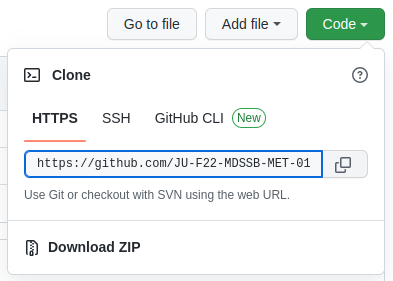
On GitHub, click on the green Code button, select HTTPS (this might already be selected by default, and if it is, you’ll see the text Use Git or checkout with SVN using the web URL). Click on the clipboard icon 📋 to copy the repo URL.
2.3 Step 2. Go to RStudio
Go to your RStudio. Select “New Project…” either from the File menu or from the special project menu on the top right of the RStudio window.

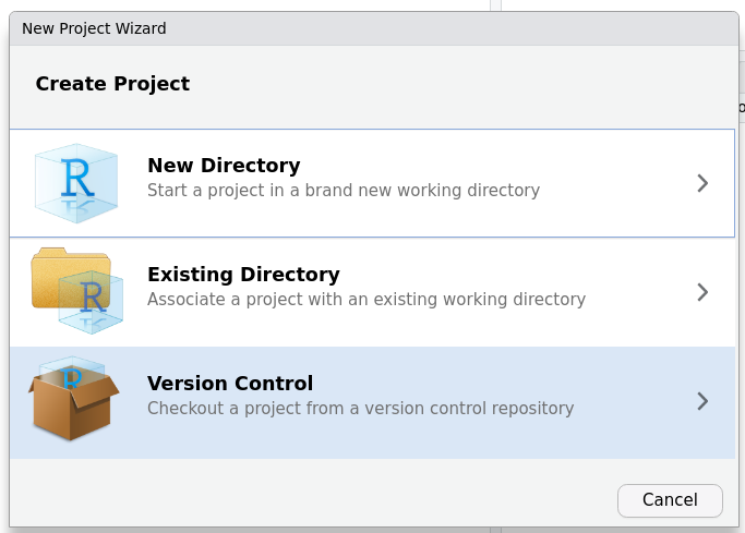
In the New Project Wizard, click on “Version Control” and then “Git”.
If “Version Control” or “Git” is not available in your RStudio, then either you haven’t installed git on you computer or your RStudio installation has not recognized it properly. In a correct installation RStudio would recognize git on your machine automatically when started. You have to solve this issue first to continue.
Then paste the repositories URL (which should still be in your clipboard) into the “Repository URL:” field. Leave directory name as it is automatically chosen, but make sure that you create the directory in a the folder where you want to store the course material on your computer via the “Browse …” button.
- Create a folder for Data Science Concepts and Tools
- Put all repos there
When you click “Create Project”
- git will create a new directory in the folder, copies all the files from github to it, and initializes your git repository locally
- RStudio will switch to that as the new project
3 Hello RStudio!
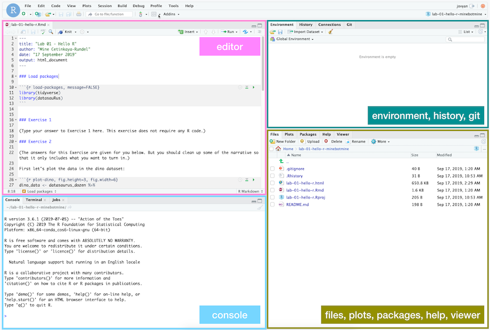
RStudio is comprised of four panes.

- On the bottom left is the Console which we already used, this is where you can write code that will be evaluated (REPL in a CLI = Read–eval–print loop in a Command Line Interface). Try typing
2 + 2here and hit enter, what do you get? - On the bottom right is the Files pane, as well as other panes that will come handy as we start our analysis.
- If you click on a file, it will open in the editor, on the top left pane.
- Finally, the top right pane shows your Environment. If you define a variable it would show up there. Try typing
x <- 2in the Console and hit enter, what do you get in the Environment pane? Importantly, this pane is also where the Git interface lives. We will be using that regularly throughout this assignment.
4 Warm up
Before we introduce the data, let’s warm up with some simple exercises.
The top portion of your quarto file (between the three dashed lines) is called YAML. It stands for “YAML Ain’t Markup Language”. It is a human friendly data serialization standard for all programming languages. All you need to know is that this area is called the YAML (we will refer to it as such) and that it contains meta information about your document.
4.1 Step 1. Update the YAML
Open the quarto (qmd) file in your project. In the YAML change the author name to your name, and “Render” the document.
 This calls
 quarto, and quarto renders the document. In this case, that means, quarto creates a new file “hw-01-R.md” in the html format as specified in the YAML.
When the file was rendered successfully, RStudio shows it in the “Viewer” pane at the bottom right. At the same place you can look in the “Files” pane you can check if the file is there. You can click on it an select to show it in your Brwoser.
Now you see a nice html-page in the Browser! You made a page like every ordinary site on the internet. So you made an important step towards publishing you data science work on the internet. However now the html page is only locally on your computer.
If you do not find the “Render” button in your RStudio installation, then either quarto is not installed or RStudio has not recognized. You have to fix this issue first before you can continue. Another source of error while rendering could be that you haven’t installed the tidyverse package.
4.2 Step 2: Commit
Go to the Git pane in your RStudio (top right corner).
You should see that your qmd (quarto) file and its output, your html-file, are listed there as recently changed files.
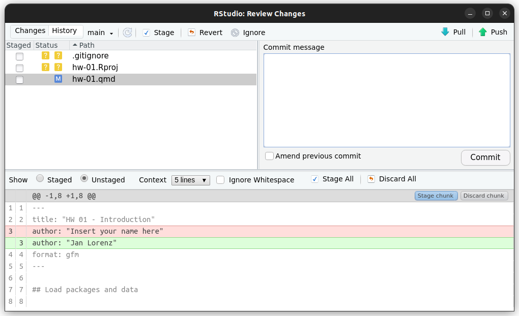
Next, click on Diff. This will pop open a new window that shows you the difference between the last committed state of the document and its current state that includes your changes. (Click on the file “hw-01-R.qmd”.) If you’re happy with these changes, click on the checkboxes of all files in the list, and type “Update author name” in the Commit message box and hit Commit and then close the window.

You don’t have to commit after every change, this would get quite cumbersome. You should consider committing states that are meaningful to you for inspection, comparison, or restoration. In the first few assignments we may tell you exactly when to commit and what commit message to use. As the semester progresses we will let you make these decisions.
4.3 Step 3. Push
Now that you have made an update and committed this change, it’s time to push these changes to the web! Or more specifically, to your repo on GitHub.
Why?
So that others can see your changes.
And by others, we mean the course instructors (your repos in this course are private to you and us, only).
Go the Git pane and click on Push.
Thought exercise: Which of the steps “updating the YAML”, “committing”, and “pushing” involves talking to GitHub?1
4.4 Check what you did
Go to your repository on https://github.com/JU-F22-MDSSB-MET-01 and check if the files appear there as in you local folder.
- You may wonder why clicking on the the html-file does not show the page as you saw it locally in your browser.
- The reason is, that GitHub is essentially a code editor. So, it shows you the html-code. This code was created by rendering. DO not touch it “by hand”. It will be overwritten every time you render again.
- Viewing the html as in the browser is not possible here. The instructor will clone you repository and can then look at your html locally on their machines.
- Context Information: It is possible to publish webpages from GitHub. You can learn this later.
- Context Information: GitHub provides its own gfm = GitHub Flavoured Markdown. The README.md files are written in this. gfm is very similar to the Markdown language we use.
5 Packages
R is an open-source language, and developers contribute functionality to R via packages.
In this assignment we will use the following packages tidyverse, a collection of packages for doing data analysis in a “tidy” way.
We use the library() function to load packages.
We use the function read_csv from the tidyverse package readr to read the data in the csv-file “data/ourdatascienceprofiles.csv” which we produced during the first lecture.
In your R Markdown document you should see an R chunk labelled load-packages-and-data which has the necessary code for loading packages and data.
You should also load these packages in your Console, which you can do by sending the code to your Console by clicking on the Run Current Chunk icon (small green triangle pointing right icon).

- This is a typical source of confusion.
- When you execute code in the Console objects will be created in your working environment. See the Environment Tab.
- When you render the qmd-file to html, quarto creates a new environment and goes through all the code in the code chunks step by step in an own rendering environment. It can not access, and does not know what you created in the working environment!
- How to use it properly: When you develop code you send code lines to the console repeatedly to workout how your code works. However you have to take care that the code writte there is complete in the right order, that quarto can then do the necessary steps to reproduce what you want it to do.
- You will get used to this workflow.
6 Data
The dataset is now visible under the name profiles in your Environment pane (top right area). You can view the dataset as a spreadsheet using the View() function.
Note that you should not put this function in your R Markdown document, but instead type it directly in the Console, as it pops open a new window (and the concept of popping open a window in a static document doesn’t really make sense…).
When you run this in the console, you’ll see the data viewer window pop up. You can also write the object name profiles to the console and get a brief outlook of the data, or you can take a glimpse to get meta-information about dimensions, variable names, and data types. Try all in the Console.
View(profiles)
profiles
glimpse(profiles)
7 Graphic
There is another chunk called my-data-science-profile. It has code which
- tidies the data by making it longer and less wide such that the data from the seven dimensions, go to two variables “Dimension” and “value”.
- filters the data of one person
- makes a graphic which is called a barplot of the data science profile of that person
Run the code in this chunk in the Console and see how the Plots pane pops up to show the graphic.
8 Exercises
- Show your data science profile!
Change the code in the my-data-science-profile chunk such that it shows your profile. Render the document, commit your changes with a commit message that says “Completed Exercise 1”, and push to GitHub. Make sure to commit and push all changed files so that your Git pane is cleared up afterwards.
If you haven’t entered your data during class, then use the name of another person in the dataset. If you want to have your data included then you can still fill out the survey https://forms.office.com/e/Uz84tQVNWQ. We will update the dataset later and inform you when it is ready. For now you have to choose another name.
- Write a short text about your data science profile going through the dimensions and tell what is behind that value.
Write your text under the my-data-science-profile chunk. Format some words in bold or italic, e.g., the dimension names. You can find the formatting basic of markdown in quarto here: https://quarto.org/docs/authoring/markdown-basics.html. Render the document, commit with message “Completed Exercise 2”, and push. You can check on GitHub if the file “hw-01-R.md” looks good in the browser.
- Averaging over all people, what is the Dimension with the most and the least experience in the group?
Copy this code to your Console and read the output:
profiles |>
  summarize(across(`Social Science`:`Machine Learning`, mean))
Copy the code and write your answer into the outlined places in the document.
- How many in the group work on Windows, Mac, and Linux?
Copy this code to your Console and read the output:
profiles |>
  group_by(`What is the operating system of your computer?`) |>
  count()
Copy the code and write your answer into the outlined places in the document.
Render the document, commit with message “Completed up to Exercise 4”, and push. Check on GitHub that the file “hw-01-R.md” looks good in the browser.
- How is the experience with AI Tools in the group?
This is a more open exercise. Think about how you would like to view this data and try to produce a graphic for each of the three question. Each question would have a new chunk. Try to draft a graphic. Try the geom_bar aesthetic. When your graphs are read, write short text before each graphic and a short summary about the question after all three graphics. Look at the html-output. Can readers extract your insights convincingly?
Footnotes
Only the push talks to GitHub. Editing and committing happens on your local machine.↩︎