W#09: Hypothesis Testing

Jan Lorenz

Hypothesis testing

Large part of the content adapted from http://datasciencebox.org.

Organ donors

People providing an organ for donation sometimes seek the help of a special “medical consultant”. These consultants assist the patient in all aspects of the surgery, with the goal of reducing the possibility of complications during the medical procedure and recovery. Patients might choose a consultant based in part on the historical complication rate of the consultant’s clients.

One consultant tried to attract patients by noting that the average complication rate for liver donor surgeries in the US is about 10%, but her clients have only had 3 complications in the 62 liver donor surgeries she has facilitated. She claims this is strong evidence that her work meaningfully contributes to reducing complications (and therefore she should be hired!).

Data

organ_donor <- tibble(
  outcome = c(rep("complication", 3), rep("no complication", 59))
)

organ_donor |>
  count(outcome)

# A tibble: 2 × 2
  outcome             n
  <chr>           <int>
1 complication        3
2 no complication    59

Parameter vs. statistic

A parameter for a hypothesis test is the “true” value of interest. We typically estimate the parameter using a sample statistic as a point estimate.

\(p\): true rate of complication, here 0.1 (10% complication rate in US)

\(\hat{p}\): rate of complication in the sample = \(\frac{3}{62}\) = 0.048 (This is the point estimate.)

Correlation vs. causation

Is it possible to infer the consultant’s claim using the data?

No. The claim is: There is a causal connection. However, the data are observational. For example, maybe patients who can afford a medical consultant can afford better medical care, which can also lead to a lower complication rate (for example).

While it is not possible to assess the causal claim, it is still possible to test for an association using these data. For this question we ask, could the low complication rate of \(\hat{p}\) = 0.048 be due to chance?

Two claims

• Null hypothesis: “There is nothing going on”

Complication rate for this consultant is no different than the US average of 10%

• Alternative hypothesis: “There is something going on”

Complication rate for this consultant is lower than the US average of 10%

Hypothesis testing as a court trial

• Null hypothesis, \(H_0\): Defendant is innocent

• Alternative hypothesis, \(H_A\): Defendant is guilty

• Present the evidence: Collect data

• Judge the evidence: “Could these data plausibly have happened by chance if the null hypothesis were true?”

  • Yes: Fail to reject \(H_0\)
  • No: Reject \(H_0\)

Hypothesis testing framework

• Start with a null hypothesis, \(H_0\), that represents the status quo

• Set an alternative hypothesis, \(H_A\), that represents the research question, i.e. what we are testing for

• Conduct a hypothesis test under the assumption that the null hypothesis is true and calculate a p-value.
  Definition p-value: Probability of observed or more extreme outcome given that the null hypothesis is true.

  • if the test results suggest that the data do not provide convincing evidence for the alternative hypothesis, stick with the null hypothesis
  • if they do, then reject the null hypothesis in favor of the alternative

Setting the hypotheses

Which of the following is the correct set of hypotheses for the claim that the consultant has lower complication rates?

1. \(H_0: p = 0.10\); \(H_A: p \ne 0.10\)

2. \(H_0: p = 0.10\); \(H_A: p > 0.10\)

3. \(H_0: p = 0.10\); \(H_A: p < 0.10\)

4. \(H_0: \hat{p} = 0.10\); \(H_A: \hat{p} \ne 0.10\)

5. \(H_0: \hat{p} = 0.10\); \(H_A: \hat{p} > 0.10\)

6. \(H_0: \hat{p} = 0.10\); \(H_A: \hat{p} < 0.10\)

Correct is c. Hypotheses are about the true rate of complication \(p\) not the observed ones \(\hat{p}\)

Simulating the null distribution

Since \(H_0: p = 0.10\), we need to simulate a null distribution where the probability of success (complication) for each trial (patient) is 0.10.

How should we simulate the null distribution for this study using a bag of chips?

• How many chips? For example 10 which makes 10% choices possible
• How many colors? 2
• What should colors represent? “complication”, “no complication”
• How many draws? 62 as the data
• With replacement or without replacement? With replacement

When sampling from the null distribution, what would be the expected proportion of “complications”? 0.1

Simulation!

set.seed(1234)
outcomes <- c("complication", "no complication")
sim1 <- sample(outcomes, size = 62, prob = c(0.1, 0.9), replace = TRUE)
sim1

 [1] "no complication" "no complication" "no complication" "no complication"
 [5] "no complication" "no complication" "no complication" "no complication"
 [9] "no complication" "no complication" "no complication" "no complication"
[13] "no complication" "complication"    "no complication" "no complication"
[17] "no complication" "no complication" "no complication" "no complication"
[21] "no complication" "no complication" "no complication" "no complication"
[25] "no complication" "no complication" "no complication" "complication"   
[29] "no complication" "no complication" "no complication" "no complication"
[33] "no complication" "no complication" "no complication" "no complication"
[37] "no complication" "no complication" "complication"    "no complication"
[41] "no complication" "no complication" "no complication" "no complication"
[45] "no complication" "no complication" "no complication" "no complication"
[49] "no complication" "no complication" "no complication" "no complication"
[53] "no complication" "no complication" "no complication" "no complication"
[57] "no complication" "no complication" "no complication" "no complication"
[61] "no complication" "no complication"

sum(sim1 == "complication")/62

[1] 0.0483871

Oh OK, this was is pretty close to the consultant’s rate. But maybe it was a rare event?

More simulation!

one_sim <- function() sample(outcomes, size = 62, prob = c(0.1, 0.9), replace = TRUE)

sum(one_sim() == "complication")/62

[1] 0.1290323

sum(one_sim() == "complication")/62

[1] 0.1290323

sum(one_sim() == "complication")/62

[1] 0.09677419

sum(one_sim() == "complication")/62

[1] 0.09677419

sum(one_sim() == "complication")/62

[1] 0.1774194

sum(one_sim() == "complication")/62

[1] 0.1129032

sum(one_sim() == "complication")/62

[1] 0.1129032

Automating with tidymodels¹

organ_donor

# A tibble: 62 × 1
   outcome        
   <chr>          
 1 complication   
 2 complication   
 3 complication   
 4 no complication
 5 no complication
 6 no complication
 7 no complication
 8 no complication
 9 no complication
10 no complication
# ℹ 52 more rows

set.seed(10)
null_dist <- organ_donor |>
  specify(response = outcome, success = "complication") |>
  hypothesize(null = "point", 
              p = c("complication" = 0.10, "no complication" = 0.90)) |> 
  generate(reps = 100, type = "draw") |> 
  calculate(stat = "prop")
null_dist

Response: outcome (factor)
Null Hypothesis: point
# A tibble: 100 × 2
   replicate   stat
       <int>  <dbl>
 1         1 0.0323
 2         2 0.0645
 3         3 0.0968
 4         4 0.0161
 5         5 0.161 
 6         6 0.0968
 7         7 0.0645
 8         8 0.129 
 9         9 0.161 
10        10 0.0968
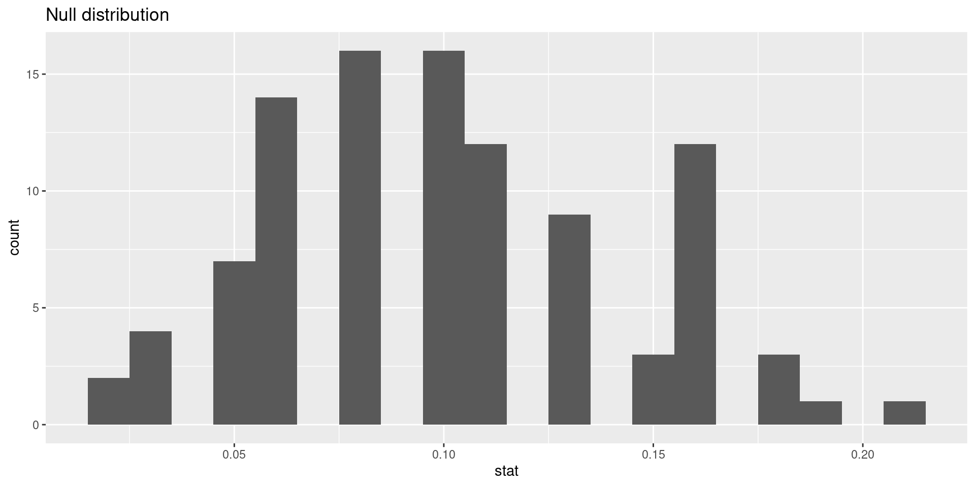
# ℹ 90 more rows

1. Of course, you can also do it in your own way without packages.

Visualizing the null distribution

ggplot(data = null_dist, mapping = aes(x = stat)) +
  geom_histogram(binwidth = 0.01) +
  labs(title = "Null distribution")

Calculating the p-value, visually

What is the p-value:¹ How often was the simulated sample proportion at least as extreme as the observed sample proportion?

ggplot(data = null_dist, mapping = aes(x = stat)) +
  geom_histogram(binwidth = 0.01) +
  labs(title = "Null distribution")  +
 geom_vline(xintercept = 3/62, color = "red")

1. The name p-value has nothing to do with the value \(p\) we are currently trying to use as population parameter.

Calculating the p-value, directly

null_dist |>
 summarise(p_value = sum(stat <= 3/62)/n())

# A tibble: 1 × 1
  p_value
    <dbl>
1    0.13

This is the fraction of simulations where complications was equal or below 0.0483871.

Significance level

• A significance level \(\alpha\) is a threshold we make up to make our judgment about the plausibility of the null hypothesis being true given the observed data.

• We often use \(\alpha = 0.05 = 5\%\) as the cutoff for whether the p-value is low enough that the data are unlikely to have come from the null model.

• If p-value < \(\alpha\), reject \(H_0\) in favor of \(H_A\): The data provide convincing evidence for the alternative hypothesis.

• If p-value > \(\alpha\), fail to reject \(H_0\) in favor of \(H_A\): The data do not provide convincing evidence for the alternative hypothesis.

What is the conclusion of the hypothesis test?

Since the p-value is greater than the significance level, we fail to reject the null hypothesis. These data do not provide convincing evidence that this consultant incurs a lower complication rate than the 10% overall US complication rate.

100 simulations is not sufficient

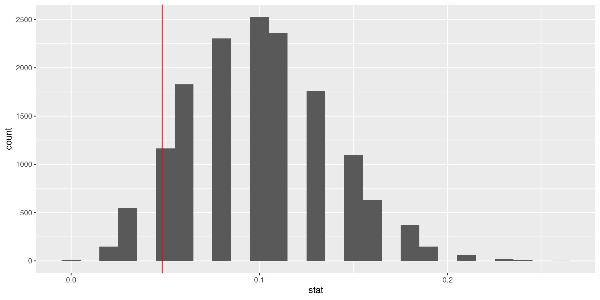
• We simulate 15,000 times to get an accurate distribution.

null_dist <- organ_donor |>
  specify(response = outcome, success = "complication") |>
  hypothesize(null = "point", 
              p = c("complication" = 0.10, "no complication" = 0.90)) |> 
  generate(reps = 15000, type = "simulate") |> 
  calculate(stat = "prop")
ggplot(data = null_dist, mapping = aes(x = stat)) +
  geom_histogram(binwidth = 0.01) +
  geom_vline(xintercept = 3/62, color = "red")

Our more robust p-value

For the null distribution with 15,000 simulations

null_dist |>
  filter(stat <= 3/62) |>
  summarise(p_value = n()/nrow(null_dist))

# A tibble: 1 × 1
  p_value
    <dbl>
1   0.125

Oh OK, our fist p-value was much more borderline in favor of the alternative hypothesis.

p-value in model outputs

Model output for a linear model with palmer penguins.

linear_reg() |> set_engine("lm") |> 
    fit(bill_length_mm ~ bill_depth_mm, data = penguins) |> tidy()

# A tibble: 2 × 5
  term          estimate std.error statistic  p.value
  <chr>            <dbl>     <dbl>     <dbl>    <dbl>
1 (Intercept)     55.1       2.52      21.9  6.91e-67
2 bill_depth_mm   -0.650     0.146     -4.46 1.12e- 5

Model output for a logistic regression model with email from openintro

logistic_reg() |>  set_engine("glm") |>
  fit(spam ~ from + cc, data = email, family = "binomial") |> tidy()

# A tibble: 3 × 5
  term         estimate std.error statistic p.value
  <chr>           <dbl>     <dbl>     <dbl>   <dbl>
1 (Intercept)  13.6      309.        0.0439   0.965
2 from1       -15.8      309.       -0.0513   0.959
3 cc            0.00423    0.0193    0.220    0.826

What do the p-values mean? What is the null hypothesis?

Null-Hypothesis: There is no relationship between the predictor variable and the response variable, that means that the coefficient is equal to zero.

Smaller the p-value \(\to\) more evidence for rejecting the hypothesis that there is no effect.

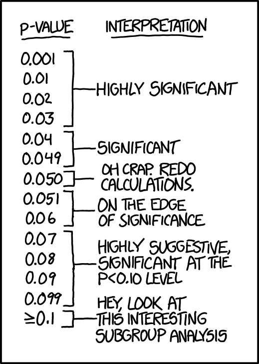
xkcd on p-values

• Significance levels are fairly arbitrary. Sometimes they are used (wrongly) as definitive judgments
• They can even be used to do p-hacking: Searching for “significant” effects in observational data
• In parts of science it has become a “gamed” performance metric.
• The p-value says nothing about effect size!

p-value misinterpretation

p-values do not measure¹

• the probability that the studied hypothesis is true
• the probability that the data were produced by random chance alone
• the size of an effect
• the importance of a result” or “evidence regarding a model or hypothesis” (it is only against the null hypothesis).

Correct:
The p-value is the probability of obtaining test results at least as extreme as the result actually observed, under the assumption that the null hypothesis is correct.

p-values and significance tests, when properly applied and interpreted, increase the rigor of the conclusions drawn from data.²

1. From the American Statistical Association (ASA) 2016

2. From the American Statistical Association (ASA) 2019