parsnip model object
Call:
stats::lm(formula = flipper_length_mm ~ body_mass_g, data = data)
Coefficients:
(Intercept) body_mass_g
136.72956 0.01528 W#07: Fitting Linear Models, Interaction Effects, Nonlinear Models, Predicting Categorical Variables
Fitting Models (Part 2)
Today: The linear model.
Recap: Linear model
Flipper length as a function of body mass.
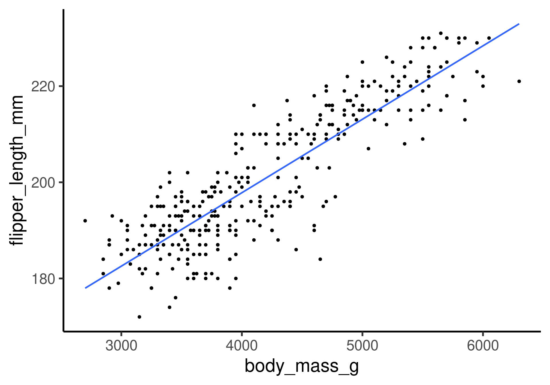
The fitting question: How can we get this line?
Recap: A line
A line is a shift-scale transformation of the identity function usually written in the form
\[f(x) = a\cdot x + b\]
where \(a\) is the slope, \(b\) is the intercept.

Recap: Terminology
- Response variable:1 Variable whose behavior or variation you are trying to understand, on the y-axis
- Explanatory variable(s):2 Other variable(s) that you want to use to explain the variation in the response, on the x-axis
- Predicted value: Output of the model function.
- The model function gives the (expected) average value of the response variable conditioning on the explanatory variables
- Residual(s): A measure of how far away a case is from its predicted value (based on the particular model)
Residual = Observed value - Predicted value
The residual tells how far above/below the expected value each case is
Our goal
Predict flipper length from body mass
average flipper_length_mm \(= \beta_0 + \beta_1\cdot\) body_mass_g
\(\beta_0\) is the intercet of the line
\(\beta_1\) is the slope of the line
Later we will have \(\beta_2, \dots, \beta_m\) as coefficients for more variables.
Fitting the model in R
average flipper_length_mm \(= 136.72956 + 0.01528\cdot\) body_mass_g
Interpretation:
The penguins have a flipper length of 136.7 mm plus 0.01528 mm for each gram of body mass (that is 15.28 mm per kg). Penguins with zero mass have a flipper length of 136.7 mm. However, this is not in the range where the model was fitted.
parsnip model objects
pengmod <- linear_reg() |>
set_engine("lm") |>
fit(flipper_length_mm ~ body_mass_g, data = penguins)
class(pengmod) # attributes[1] "_lm" "model_fit"[1] "list"[1] "lvl" "spec" "fit" "preproc" "elapsed"
[6] "censor_probs"Most interesting for us for now: $fit
Notice: parsnip model object is now missing in the output.
$fit is the object created by lm (base R)
[1] "coefficients" "residuals" "effects" "rank"
[5] "fitted.values" "assign" "qr" "df.residual"
[9] "na.action" "xlevels" "call" "terms"
[13] "model" stats::lm(formula = flipper_length_mm ~ body_mass_g, data = data) (Intercept) body_mass_g
136.72955927 0.01527592 1 2 3 5 6 7
194.0142 194.7780 186.3763 189.4315 192.4867 192.1048 1 2 3 5 6 7
-13.014243 -8.778039 8.623715 3.568532 -2.486651 -11.104753 Fitting method: Least squares regression
- The regression line shall minimize the sum of the squared residuals
(or, identically, their mean). - Mathematically: The residual for case \(i\) is \(e_i = \hat y_i - y_i\).
- Now we want to minimize \(\sum_{i=1}^n e_i^2\)
(or equivalently \(\frac{1}{n}\sum_{i=1}^n e_i^2\) the the mean of squared errors, which we will look at later).
Visualization of residuals
The residuals are the gray lines between predictid values on the regression line and the actual values.

Check: Fitted values and Residuals
Recall: Residual = Observed value - Predicted value
The Predicted values are also called Fitted values. Hence:
Residuals + Fitted values = Observed values
Proporties of least squares regression
The regression lines goes through the point (mean(x), mean(y)).
[1] 4201.754[1] 200.9152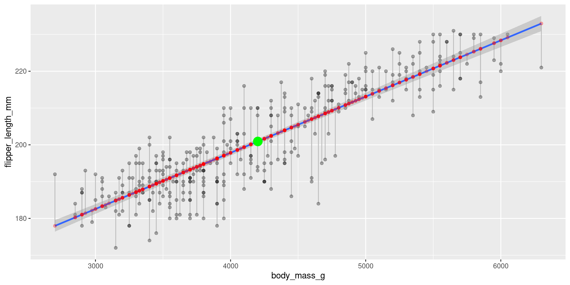
Proporties of least squares regression
Residuals sum up to zero
pengmod <- linear_reg() |> set_engine("lm") |> fit(flipper_length_mm ~ body_mass_g, data = penguins)
pengmod$fit$residuals |> sum()[1] -3.765044e-14There is no correlation between residuals and the explanatory variable
The correlation of \(x\) and \(y\) is the slope \(\beta_1\) corrected by their standard deviations.
correlation <- cor(penguins$flipper_length_mm, penguins$body_mass_g, use = "pairwise.complete.obs")
sd_flipper <- sd(penguins$flipper_length_mm, na.rm = T)
sd_mass <- sd(penguins$body_mass_g, na.rm = T)
c(correlation, sd_flipper, sd_mass)[1] 0.8712018 14.0617137 801.9545357[1] 0.01527592 (Intercept) body_mass_g
136.72955927 0.01527592 Correlation and linear regression
When the two variables in the linear regression are standardized (standard scores)
- the intercept is zero
- the coefficient coincides with the correlation
Linear Models and Dummy Variables
Explanatory variables are categorical
Let’s just try what happens with species as explanatory variable. Remember, we have three species: Adelie, Chinstrap, Gentoo.
# A tibble: 3 × 5
term estimate std.error statistic p.value
<chr> <dbl> <dbl> <dbl> <dbl>
1 (Intercept) 190. 0.540 351. 0
2 speciesChinstrap 5.87 0.970 6.05 3.79e- 9
3 speciesGentoo 27.2 0.807 33.8 1.84e-110What happened?
Two of the three species categories appear as variables now.
- Categorical variables are automatically encoded to dummy variables
- Each coefficient describes the expected difference between flipper length of that particular species compared to the baseline level
- What is the baseline level? The first category! (Here alphabetically
"Adelie")
How do dummy variables look?
| species | speciesChinstrap | speciesGentoo |
|---|---|---|
| Adelie | 0 | 0 |
| Chinstrap | 1 | 0 |
| Gentoo | 0 | 1 |
Then the fitting of the linear model is as before using the zero-one variables.
Interpretation
# A tibble: 3 × 5
term estimate std.error statistic p.value
<chr> <dbl> <dbl> <dbl> <dbl>
1 (Intercept) 190. 0.540 351. 0
2 speciesChinstrap 5.87 0.970 6.05 3.79e- 9
3 speciesGentoo 27.2 0.807 33.8 1.84e-110- Flipper length of the baseline species is the intercept.
- Average flipper length of Adelie is 190 mm
- Flipper length of the two other species add their coefficient
- Average flipper length of Chinstrap is 190 + 5.87 mm
- Average flipper length of Gentoo is 190 + 27.2 mm
Compare to a visualization
# A tibble: 3 × 5
term estimate std.error statistic p.value
<chr> <dbl> <dbl> <dbl> <dbl>
1 (Intercept) 190. 0.540 351. 0
2 speciesChinstrap 5.87 0.970 6.05 3.79e- 9
3 speciesGentoo 27.2 0.807 33.8 1.84e-110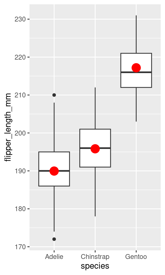
The red dots are the average values for species.
Linear models and R-squared
Linear model
# A tibble: 2 × 5
term estimate std.error statistic p.value
<chr> <dbl> <dbl> <dbl> <dbl>
1 (Intercept) 137. 2.00 68.5 5.71e-201
2 body_mass_g 0.0153 0.000467 32.7 4.37e-107average flipper_length_mm \(= 137 + 0.0153\cdot\) body_mass_g
# A tibble: 2 × 5
term estimate std.error statistic p.value
<chr> <dbl> <dbl> <dbl> <dbl>
1 (Intercept) 20.9 0.844 24.7 4.72e-78
2 bill_length_mm -0.0850 0.0191 -4.46 1.12e- 5average bill_depth_mm \(= 20.9 -0.085\cdot\) bill_length_mm
Technical: The idea of the tidy() function is to turn an object into a tidy tibble. Here, it extracts the coefficients of the linear model (and more statistical information).
R-squared of a fitted model
\(R^2\) is the percentage of variability in the response explained by the regression model.
R-squared is also called coefficient of determination.
Definition:
\(R^2 = 1 - \frac{SS_\text{res}}{SS_\text{tot}}\)
where \(SS_\text{res} = \sum_i(y_i - f_i)^2 = \sum_i e_i^2\) is the sum of the squared residuals, and
\(SS_\text{tot} = \sum_i(y_i - \bar y)^2\) the total sum of squares which is proportional to the variance of \(y\). (\(\bar y\) is the mean of \(y\).)
Linear model R-squared
linear_reg() |>
    set_engine("lm") |>
fit(flipper_length_mm ~ body_mass_g, data = penguins) |>
glance() # glance shows summary statistics of model fit# A tibble: 1 × 12
r.squared adj.r.squared sigma statistic p.value df logLik AIC BIC
<dbl> <dbl> <dbl> <dbl> <dbl> <dbl> <dbl> <dbl> <dbl>
1 0.759 0.758 6.91 1071. 4.37e-107 1 -1146. 2297. 2309.
# ℹ 3 more variables: deviance <dbl>, df.residual <int>, nobs <int>Interpretation R-squared? 75.9% of the variance of flipper length can be explained by a linear relation with body mass.
linear_reg() |> set_engine("lm") |>
fit(bill_depth_mm ~ bill_length_mm, data = penguins) |>
glance()# A tibble: 1 × 12
r.squared adj.r.squared sigma statistic p.value df logLik AIC BIC
<dbl> <dbl> <dbl> <dbl> <dbl> <dbl> <dbl> <dbl> <dbl>
1 0.0552 0.0525 1.92 19.9 0.0000112 1 -708. 1422. 1433.
# ℹ 3 more variables: deviance <dbl>, df.residual <int>, nobs <int>5.52% of the variance of bill depth can be explained by a linear relation with bill length.
Technical: The idea of the glance() function is to construct a single row summary “glance” of a model, fit, or other object.
R-squared and correlation
For a linear model with one predictor, the square of the correlation coefficient is the same as the R-squared of the model.
linear_reg() |> set_engine("lm") |>
fit(flipper_length_mm ~ body_mass_g, data = penguins) |>
glance()# A tibble: 1 × 12
r.squared adj.r.squared sigma statistic p.value df logLik AIC BIC
<dbl> <dbl> <dbl> <dbl> <dbl> <dbl> <dbl> <dbl> <dbl>
1 0.759 0.758 6.91 1071. 4.37e-107 1 -1146. 2297. 2309.
# ℹ 3 more variables: deviance <dbl>, df.residual <int>, nobs <int>[1] 0.7589925Hence, the name \(R^2\)!
Linear models with more predictors
More predictors: Coefficients
# A tibble: 2 × 5
  term        estimate std.error statistic   p.value
  <chr>          <dbl>     <dbl>     <dbl>     <dbl>
1 (Intercept) 137.      2.00          68.5 5.71e-201
2 body_mass_g 0.0153 0.000467 32.7 4.37e-107linear_reg() |> set_engine("lm") |>
fit(flipper_length_mm ~ body_mass_g + bill_length_mm, data = penguins) |>
tidy()# A tibble: 3 × 5
term estimate std.error statistic p.value
<chr> <dbl> <dbl> <dbl> <dbl>
1 (Intercept) 122. 2.86 42.7 1.70e-138
2 body_mass_g 0.0131 0.000545 23.9 7.56e- 75
3 bill_length_mm 0.549 0.0801 6.86 3.31e- 11linear_reg() |> set_engine("lm") |>
fit(flipper_length_mm ~ body_mass_g + bill_length_mm + bill_depth_mm, data = penguins) |>
tidy()# A tibble: 4 × 5
term estimate std.error statistic p.value
<chr> <dbl> <dbl> <dbl> <dbl>
1 (Intercept) 158. 4.63 34.1 1.80e-111
2 body_mass_g 0.0109 0.000538 20.3 1.93e- 60
3 bill_length_mm 0.592 0.0717 8.26 3.42e- 15
4 bill_depth_mm -1.68 0.181 -9.29 1.99e- 18More predictors: glance R-squared
linear_reg() |> set_engine("lm") |>
    fit(flipper_length_mm ~ body_mass_g, data = penguins) |>
 glance()
# A tibble: 1 × 12
r.squared adj.r.squared sigma statistic p.value df logLik AIC BIC
<dbl> <dbl> <dbl> <dbl> <dbl> <dbl> <dbl> <dbl> <dbl>
1 0.759 0.758 6.91 1071. 4.37e-107 1 -1146. 2297. 2309.
# ℹ 3 more variables: deviance <dbl>, df.residual <int>, nobs <int>linear_reg() |> set_engine("lm") |>
fit(flipper_length_mm ~ body_mass_g + bill_length_mm, data = penguins) |>
glance()# A tibble: 1 × 12
r.squared adj.r.squared sigma statistic p.value df logLik AIC BIC
<dbl> <dbl> <dbl> <dbl> <dbl> <dbl> <dbl> <dbl> <dbl>
1 0.788 0.787 6.49 631. 4.88e-115 2 -1123. 2255. 2270.
# ℹ 3 more variables: deviance <dbl>, df.residual <int>, nobs <int>linear_reg() |> set_engine("lm") |>
fit(flipper_length_mm ~ body_mass_g + bill_length_mm + bill_depth_mm, data = penguins) |>
glance()# A tibble: 1 × 12
r.squared adj.r.squared sigma statistic p.value df logLik AIC BIC
<dbl> <dbl> <dbl> <dbl> <dbl> <dbl> <dbl> <dbl> <dbl>
1 0.831 0.830 5.80 556. 2.99e-130 3 -1084. 2179. 2198.
# ℹ 3 more variables: deviance <dbl>, df.residual <int>, nobs <int>More predictors: Equations
average flipper_length_mm \(= 137 + 0.0153\cdot\) body_mass_g
75.9% explained variance
average flipper_length_mm \(= 122 + 0.0131\cdot\) body_mass_g \(+ 0.549\cdot\) bill_length_mm
78.8% explained variance
average flipper_length_mm \(= 158 + 0.0109\cdot\) body_mass_g \(+ 0.592\cdot\) bill_length_mm \(- 1.68\cdot\) bill_length_mm
83.1% explained variance
Adding a categorical variable as main effect
linear_reg() |> set_engine("lm") |>
 fit(flipper_length_mm ~ body_mass_g + species, data = penguins) |>
 tidy()
# A tibble: 4 × 5
term estimate std.error statistic p.value
<chr> <dbl> <dbl> <dbl> <dbl>
1 (Intercept) 159. 2.39 66.6 2.45e-196
2 body_mass_g 0.00840 0.000634 13.3 1.40e- 32
3 speciesChinstrap 5.60 0.788 7.10 7.33e- 12
4 speciesGentoo 15.7 1.09 14.4 6.80e- 37A main effect by categorical dummy variables allows for different intercepts per species. (However, the slopes are the same.)
linear_reg() |> set_engine("lm") |>
 fit(flipper_length_mm ~ body_mass_g + species, data = penguins) |>
 glance()
# A tibble: 1 × 12
r.squared adj.r.squared sigma statistic p.value df logLik AIC BIC
<dbl> <dbl> <dbl> <dbl> <dbl> <dbl> <dbl> <dbl> <dbl>
1 0.854 0.853 5.40 659. 7.42e-141 3 -1060. 2129. 2149.
# ℹ 3 more variables: deviance <dbl>, df.residual <int>, nobs <int>Adding species increases R-squared better than adding bill length and bill depth together!
Adding as interaction effect
linear_reg() |> set_engine("lm") |>
 fit(flipper_length_mm ~ body_mass_g * species, data = penguins) |>
 tidy()
# A tibble: 6 × 5
term estimate std.error statistic p.value
<chr> <dbl> <dbl> <dbl> <dbl>
1 (Intercept) 165. 3.55 46.5 1.56e-148
2 body_mass_g 0.00668 0.000952 7.01 1.30e- 11
3 speciesChinstrap -13.9 7.30 -1.90 5.84e- 2
4 speciesGentoo 6.06 6.05 1.00 3.17e- 1
5 body_mass_g:speciesChinstrap 0.00523 0.00195 2.68 7.66e- 3
6 body_mass_g:speciesGentoo 0.00236 0.00135 1.75 8.16e- 2- Note the
*for interaction effect! - Also main effects for both variables are in as coefficients.
- Adelie is the baseline species (because it is first in the alphabet).
- An interaction effect allows for different slopes for each species!
Improvement through the interaction effects is small here
linear_reg() |> set_engine("lm") |>
 fit(flipper_length_mm ~ body_mass_g + species, data = penguins) |>
 glance()
# A tibble: 1 × 12
r.squared adj.r.squared sigma statistic p.value df logLik AIC BIC
<dbl> <dbl> <dbl> <dbl> <dbl> <dbl> <dbl> <dbl> <dbl>
1 0.854 0.853 5.40 659. 7.42e-141 3 -1060. 2129. 2149.
# ℹ 3 more variables: deviance <dbl>, df.residual <int>, nobs <int>linear_reg() |> set_engine("lm") |>
fit(flipper_length_mm ~ body_mass_g * species, data = penguins) |>
glance()# A tibble: 1 × 12
r.squared adj.r.squared sigma statistic p.value df logLik AIC BIC
<dbl> <dbl> <dbl> <dbl> <dbl> <dbl> <dbl> <dbl> <dbl>
1 0.857 0.855 5.35 404. 9.60e-140 5 -1056. 2125. 2152.
# ℹ 3 more variables: deviance <dbl>, df.residual <int>, nobs <int>Regression lines by species
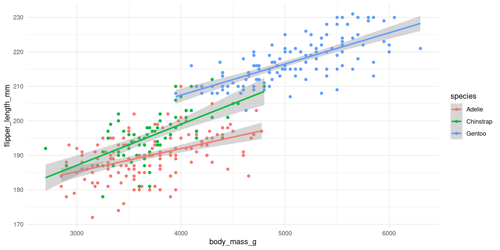
Compare the slopes to the regression output on the slides before!
Different equations for each species!
linear_reg() |> set_engine("lm") |>
 fit(flipper_length_mm ~ body_mass_g * species, data = penguins) |>
 tidy()
# A tibble: 6 × 5
term estimate std.error statistic p.value
<chr> <dbl> <dbl> <dbl> <dbl>
1 (Intercept) 165. 3.55 46.5 1.56e-148
2 body_mass_g 0.00668 0.000952 7.01 1.30e- 11
3 speciesChinstrap -13.9 7.30 -1.90 5.84e- 2
4 speciesGentoo 6.06 6.05 1.00 3.17e- 1
5 body_mass_g:speciesChinstrap 0.00523 0.00195 2.68 7.66e- 3
6 body_mass_g:speciesGentoo 0.00236 0.00135 1.75 8.16e- 2Adelie:
average flipper_length_mm \(= 165 + 0.00668\cdot\) body_mass_g
Chinstrap:
average flipper_length_mm \(= 165 - 13.6 + (0.00668 + 0.00523)\cdot\) body_mass_g
Gentoo:
average flipper_length_mm \(= 165 + 6.06 + (0.00668 + 0.00236)\cdot\) body_mass_g
Interaction effects more categoricals
Adding products of variables in the linear model \(y_i = \beta_0 + \beta_1x_1 + \beta_2x_2 + \beta_{3}x_1x_2 + \dots\).
For \(x_1\) and \(x_2\) being dummy variables for being female and having kids this is for example
| gndr_f | has_kids | gndr_f_x_has_kids |
|---|---|---|
| 0 | 1 | 0 |
| 1 | 0 | 0 |
| 1 | 1 | 1 |
| 0 | 0 | 0 |
- What is the baseline? Being male without kids.
Thought experiment:
- When we estimate a model explaining life satisfaction with these. How would we see if being a mother increases life satisfaction more than being a father? positiv coefficient for
gndr_f_x_has_kids
Nonlinear Models
When a linear model is bad
Example: Total corona cases in Germany in the first wave 2020.

\(\log\) transformation
Instead of Cumulative_cases we look at \(\log(\)Cumulative_cases\()\)
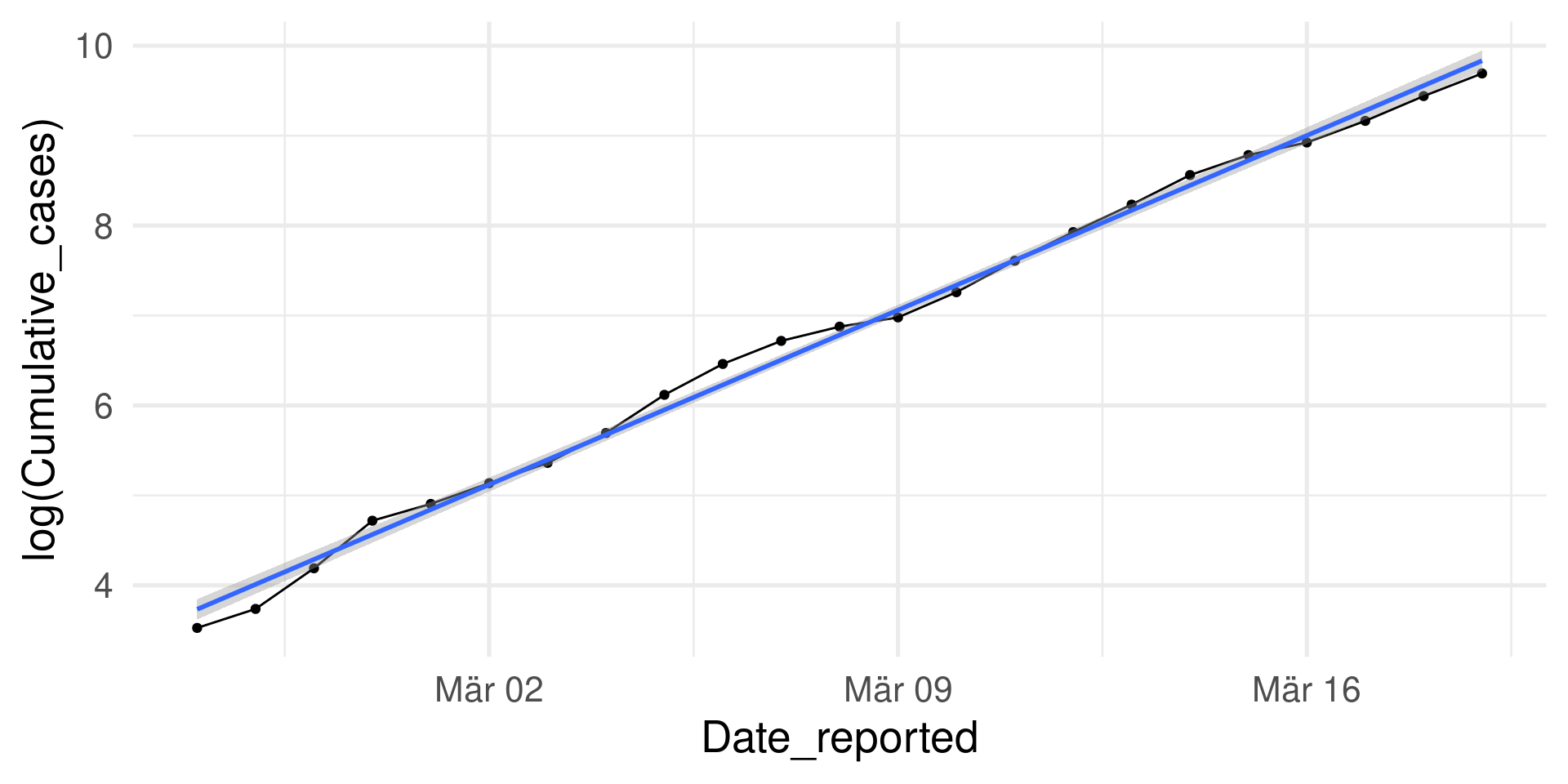
Almost perfect fit of the linear model: \(\log(y)=\log(\beta_0) + \beta_1\cdot x\)
(\(y=\) Cumulative cases, \(x=\) Days)
Exponentiation gives the model: \(y=\beta_0 e^{\beta_1\cdot x}\) (Check \(e^{\log(\beta_0) + \beta_1\cdot x} = e^{\log(\beta_0)} e^{\beta_1\cdot x} = \beta_0 e^{\beta_1\cdot x}\))
Exponential growth!
\(y=\beta_0 e^{\beta_1\cdot x}\)
For comparison: Logistic function \(y = \frac{N \beta_0 e^{\beta_1\cdot x}}{N + \beta_0 e^{\beta_1\cdot x}}\) for \(N=200000\)
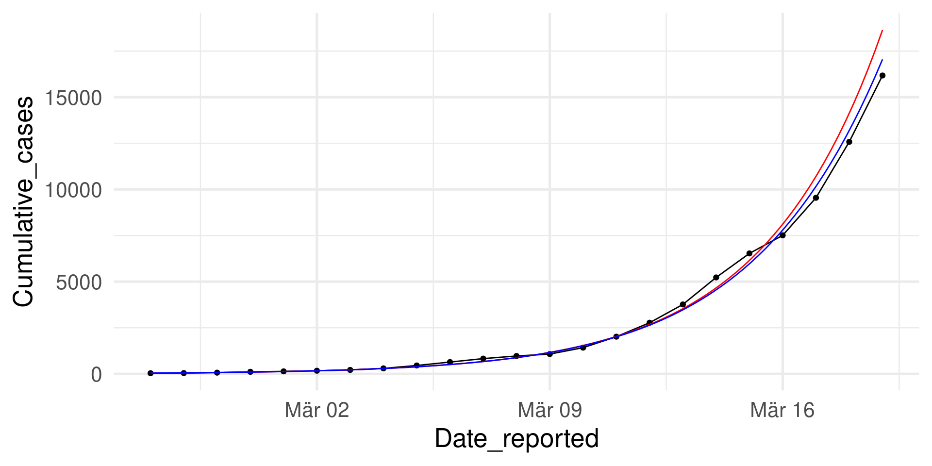
Logistic growth (as in the SI model) mimicks exponential growth initially.
\(\log\) transformation

What is the difference to the penguin model?
- \(x\) has an ordered structure and no duplicates
The fit looks so good. Why?
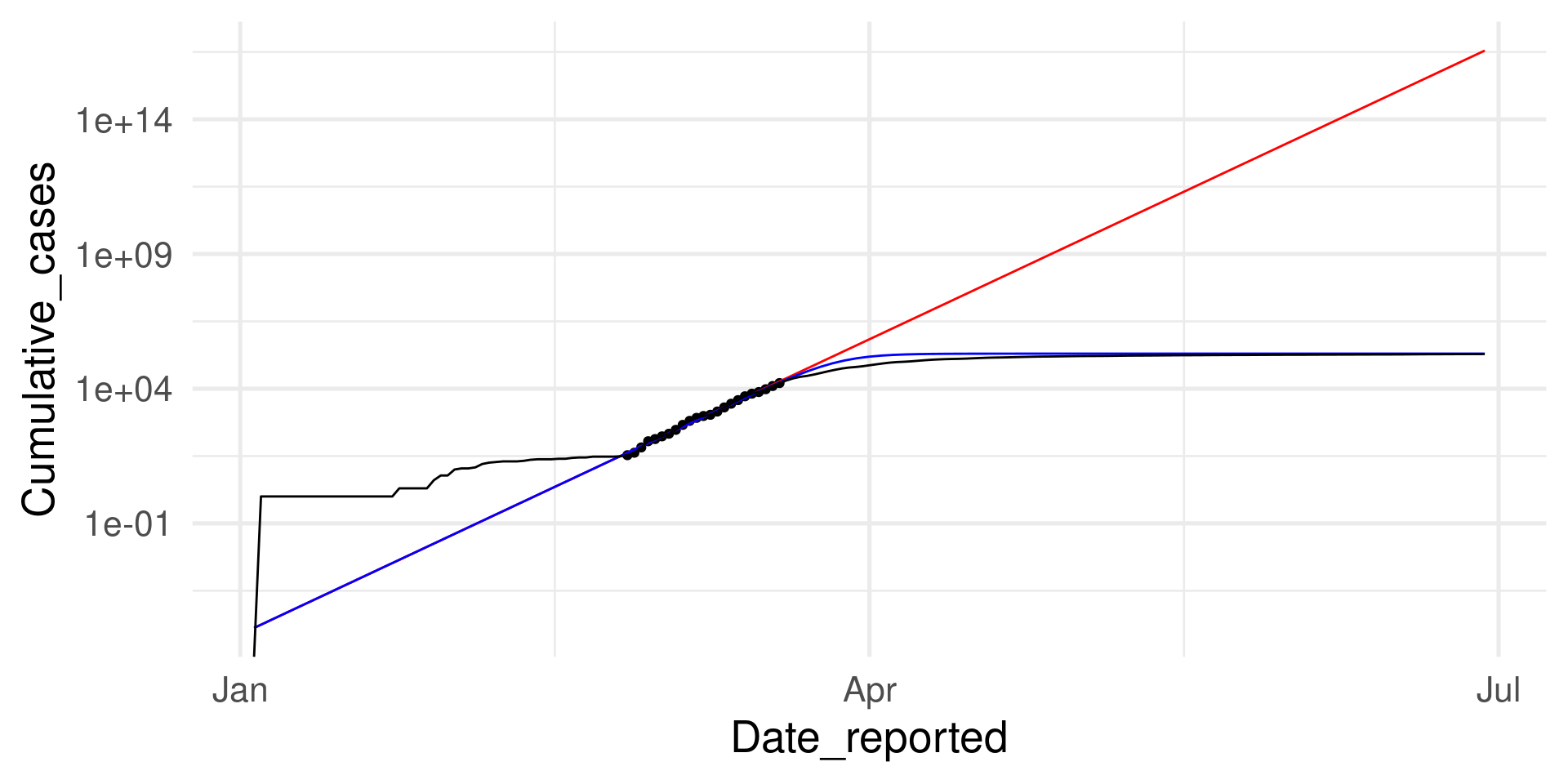
Because there is a mechanistic explanation behind: The SI model.
However, it works only in a certain range

However, it works only in a certain range (log scale on y)
Predicting Categorical Data
Large part of the content adapted from http://datasciencebox.org.
What if response is binary?
- Example: Spam filter for emails
Rows: 3,921
Columns: 21
$ spam         <fct> 0, 0, 0, 0, 0, 0, 0, 0, 0, 0, 0, 0, 0, 0, 0, 0, 0, 0, 0, …
$ to_multiple  <fct> 0, 0, 0, 0, 0, 0, 1, 1, 0, 0, 0, 0, 0, 0, 0, 0, 0, 0, 0, …
$ from         <fct> 1, 1, 1, 1, 1, 1, 1, 1, 1, 1, 1, 1, 1, 1, 1, 1, 1, 1, 1, …
$ cc           <int> 0, 0, 0, 0, 0, 0, 0, 1, 0, 0, 0, 1, 0, 1, 2, 1, 0, 2, 0, …
$ sent_email   <fct> 0, 0, 0, 0, 0, 0, 1, 1, 0, 0, 1, 0, 0, 1, 0, 1, 0, 0, 1, …
$ time         <dttm> 2012-01-01 07:16:41, 2012-01-01 08:03:59, 2012-01-01 17:…
$ image        <dbl> 0, 0, 0, 0, 0, 0, 0, 1, 0, 0, 0, 0, 0, 0, 0, 0, 0, 0, 0, …
$ attach       <dbl> 0, 0, 0, 0, 0, 0, 0, 1, 0, 0, 0, 0, 0, 0, 0, 0, 0, 0, 0, …
$ dollar       <dbl> 0, 0, 4, 0, 0, 0, 0, 0, 0, 0, 0, 0, 0, 0, 2, 0, 5, 0, 0, …
$ winner       <fct> no, no, no, no, no, no, no, no, no, no, no, no, no, no, n…
$ inherit      <dbl> 0, 0, 1, 0, 0, 0, 0, 0, 0, 0, 0, 0, 0, 0, 0, 0, 0, 0, 0, …
$ viagra       <dbl> 0, 0, 0, 0, 0, 0, 0, 0, 0, 0, 0, 0, 0, 0, 0, 0, 0, 0, 0, …
$ password     <dbl> 0, 0, 0, 0, 2, 2, 0, 0, 0, 0, 0, 0, 0, 0, 0, 0, 1, 0, 0, …
$ num_char     <dbl> 11.370, 10.504, 7.773, 13.256, 1.231, 1.091, 4.837, 7.421…
$ line_breaks  <int> 202, 202, 192, 255, 29, 25, 193, 237, 69, 68, 25, 79, 191…
$ format       <fct> 1, 1, 1, 1, 0, 0, 1, 1, 0, 1, 1, 0, 1, 1, 1, 1, 1, 1, 0, …
$ re_subj      <fct> 0, 0, 0, 0, 0, 0, 0, 0, 0, 0, 0, 1, 0, 1, 1, 1, 0, 1, 1, …
$ exclaim_subj <dbl> 0, 0, 0, 0, 0, 0, 0, 0, 0, 0, 0, 0, 0, 0, 0, 0, 1, 0, 0, …
$ urgent_subj  <fct> 0, 0, 0, 0, 0, 0, 0, 0, 0, 0, 0, 0, 0, 0, 0, 0, 0, 0, 0, …
$ exclaim_mess <dbl> 0, 1, 6, 48, 1, 1, 1, 18, 1, 0, 2, 1, 0, 10, 4, 10, 20, 0…
$ number       <fct> big, small, small, small, none, none, big, small, small, …
Multinomial response variable?
- We will not cover other categorical variables than binary ones here.
- However, many of the probabilistic concepts transfer.
Variables
?email shows all variable descriptions. For example:
spamIndicator for whether the email was spam.fromWhether the message was listed as from anyone (this is usually set by default for regular outgoing email).ccNumber of people cc’ed.timeTime at which email was sent.attachThe number of attached files.dollarThe number of times a dollar sign or the word “dollar” appeared in the email.num_charThe number of characters in the email, in thousands.re_subjWhether the subject started with “Re:”, “RE:”, “re:”, or “rE:”
Data exploration
Would you expect spam to be longer or shorter?
Would you expect spam subject to start with “Re:” or the like?
Linear models?
Both seem to give some signal. How can we model the relationship?
We focus first on just num_char:

parsnip model object


Call:
stats::lm(formula = as.numeric(spam) - 1 ~ num_char, data = data)

Coefficients:
(Intercept)     num_char
   0.118214    -0.002299
We would like to have a better concept!
A penguins example

It does not make much sense to predict 0-1-values with a linear model.
A probabilistic concept
- We treat each outcome (spam and not) as successes and failures arising from separate Bernoulli trials
- Bernoulli trial: a random experiment with exactly two possible outcomes, success and failure, in which the probability of success is the same every time the experiment is conducted
- Each email is treated as Bernoulli trial with separate probability of success
\[ y_i ∼ \text{Bernoulli}(p_i) \]
- We use the predictor variables to model the Bernoulli parameter \(p_i\)
- Now we conceptualized a continuous response, but still a linear model does not fit perfectly for \(p_i\) (since a probability is between 0 and 1).
- However, we can transform the linear model to have the appropriate range.
Generalized linear models
Characterising GLMs
- Generalized linear models (GLMs) are a way of addressing many problems in regression
- Logistic regression is one example
All GLMs have the following three characteristics:
- A probability distribution as a generative model for the outcome variable \(y_i \sim \text{Distribution}(\text{parameter})\)
- A linear model \(\eta = \beta_0 + \beta_1 X_1 + \cdots + \beta_k X_k\)
where \(\eta\) is related to a mean parameter of the distribution by the …
- Link function that relates the linear model to the parameter of the outcome distribution.


