W#06: Epidemic Modeling, Calculus, Linear Model, Fitting a Linear Model
Jan Lorenz
Epidemic Modeling
SIR model
Assume a population of \(N\) individuals.
Individuals can have different states, e.g.: Susceptible, Infectious, Recovered, …
The population divides into compartments of these states which change over time, e.g.: \(S(t), I(t), R(t)\)number of susceptible, infectious, recovered individuals
Now we define dynamics like
where the numbers on the arrows represent transition probabilities.
Agent-based Simulation
Agent-based model: Individual agents are simulated and interact with each other.
Explore and analyze with computer simulations.
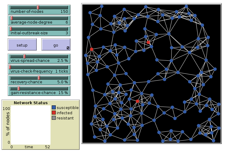
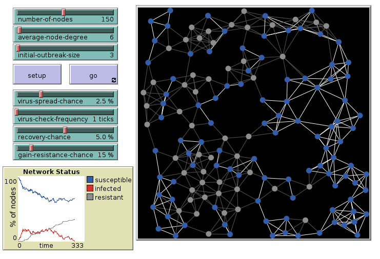
We look at the model “Virus on a Network” from the model library.
Virus on a Network: 6 links, initial
Agents connected in a network with on average 6 links per agent. 3 are infected initially.
Virus on a Network: 6 links, final
The outbreak dies out after some time.
Virus on a Network: 15 links, initial
Repeat the simulation with 15 links per agent. 3 are infected initially.
Virus on a Network: 15 links, final
The outbreak had infected most agents.
SI model
Now, we only treat the SI part of the model. We ignore recovery.
People who are susceptible can become infected through contact with infectious
People who are infectious stay infectious
The parameter \(\beta\) is the average number of contacts per unit time multiplied with the probability that an infection happens during such a contact.
SI-model: Simulation in R
We produce a vector of length \(N\) with entries representing the state of each individual as "S" or "I".
We model the random infection process in each step of unit time
Setup
Parameters: \(N=150, \beta=0.3\), a function to produce randomly infect individuals
N <-150beta <-0.3randomly_infect <-function(N, prob) { runif(N) < prob # Gives a logical vector of length N# where TRUE appears with probability beta}# Testrandomly_infect(N, beta) |>head() # First 6
[1] TRUE TRUE FALSE TRUE TRUE TRUE
init <-rep("S",N) # All susceptibleinit[1] <-"I"# Infect one individualinit |>head() # First 6
[1] "I" "S" "S" "S" "S" "S"
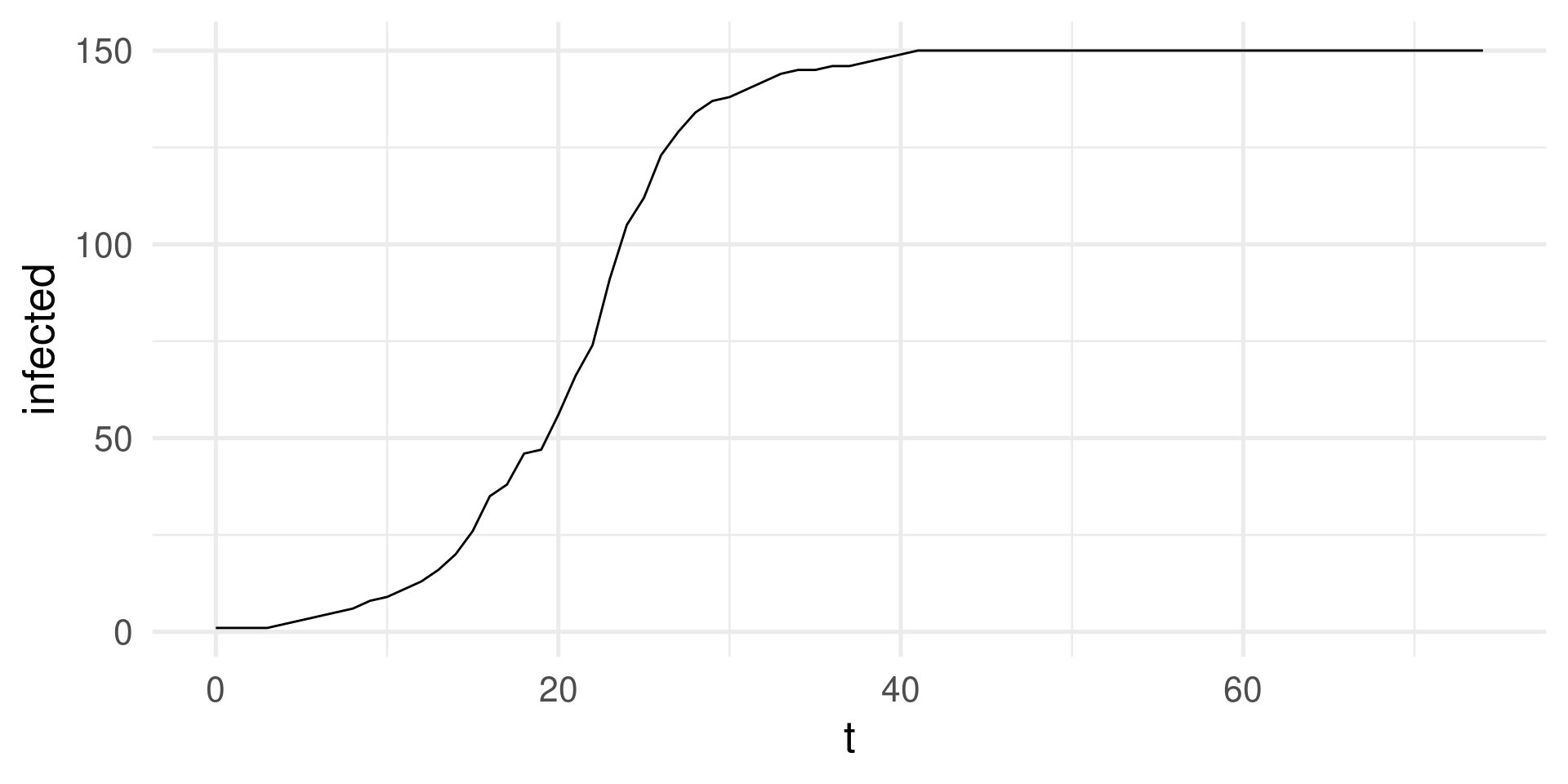
SI-model: Simulation in R
Iteration over 75 time steps.
tmax <-75sim_run <-list(init) # list with one element# This list will collect the states of # all individuals over tmax time steps for (i in2:tmax) {# Every agents has a contact with a random other contacts <-sample(sim_run[[i-1]], size = N) sim_run[[i]] <-if_else( # vectorised ifelse# conditions vector: contact is infected# and a random infection happens contacts =="I"&randomly_infect(N, beta), true ="I", false = sim_run[[i-1]] ) # otherwise state stays the same}sim_output <-tibble( # create tibble for ggplot# Compute a vector with length tmax # with the count of "I" in sim_run listt =0:(tmax-1), # times steps# count of infected, notice map_dblinfected =map_dbl(sim_run, \(x) sum(x =="I"))) sim_output |>ggplot(aes(t,infected)) +geom_line() +theme_minimal(base_size =20)
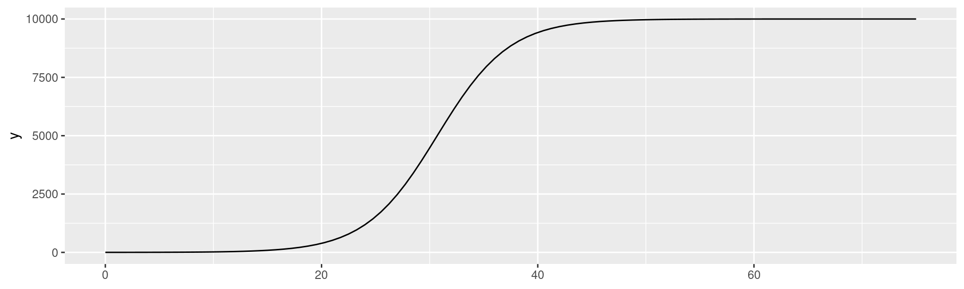
SI-model: Simulation in R
Run with \(N = 10000\)
N <-10000init <-rep("S",N) # All susceptibleinit[1] <-"I"# Infect one individualtmax <-75sim_run <-list(init) # list with one element# This list will collect the states of # all individuals over tmax time steps for (i in2:tmax) {# Every agents has a contact with a random other contacts <-sample(sim_run[[i-1]], size = N) sim_run[[i]] <-if_else( # vectorised ifelse# conditions vector: contact is infected# and a random infection happens contacts =="I"&randomly_infect(N, beta), true ="I", false = sim_run[[i-1]] ) # otherwise state stays the same}sim_output <-tibble( # create tibble for ggplot# Compute a vector with length tmax # with the count of "I" in sim_run listt =0:(tmax-1), # times steps# count of infected, notice map_dblinfected =map_dbl(sim_run, \(x) sum(x =="I"))) sim_output |>ggplot(aes(t,infected)) +geom_line() +theme_minimal(base_size =20)
New programming concepts
From base R:
runif random numbers from uniform distribution sample random sampling from a vector for loop over commands with index (i) taking values of a vector (2:tmax) one by one if_else vectorized version of conditional statements
Calculus
The mathematics of the change and the accumulation of quantities
Motivation: SI model with population compartments
Two compartments: \(S(t)\) is the number of susceptible people at time \(t\). \(I(t)\) is the number of infected people at time \(t\).
It always holds \(S(t) + I(t) = N\). (The total population is constant.)
How many infections per time?
The change of the number of infectious
\[\frac{dI}{dt} = \underbrace{\beta}_\text{infection prob.} \cdot \underbrace{\frac{S}{N}}_\text{frac. of $S$ still there} \cdot \underbrace{\frac{I}{N}}_\text{frac. $I$ to meet} \cdot N = \frac{\beta\cdot S\cdot I}{N}\]
where \(dI\) is the change of \(I\) (the newly infected here) and \(dt\) the time interval.
Interpretation: The newly infected are from the fraction of susceptible times the probability that they meet an infected times the infection probability times the total number of individuals. Same logic as our Simulation in R!
Using \(S = N - I\) we rewrite
\[\frac{dI}{dt} = \frac{\beta (N-I)I}{N}\]
Ordinary differential equation
We interpret \(I(t)\) as a function of time which gives us the number of infectious at each point in time. The change function is now
Plot the equation for \(N = 10000\), \(I_0 = 1\), and \(\beta = 0.3\)
N <-10000I0 <-1beta <-0.3ggplot() +geom_function( fun =function(t) N / (1+ (N/I0 -1)*exp(-beta*t)) ) +xlim(c(0,75))
SI-model: Numerical integration
Another way of solution using, e.g., using Euler’s method.
We compute the solution step-by-step using increments of, e.g. \(dt = 1\).
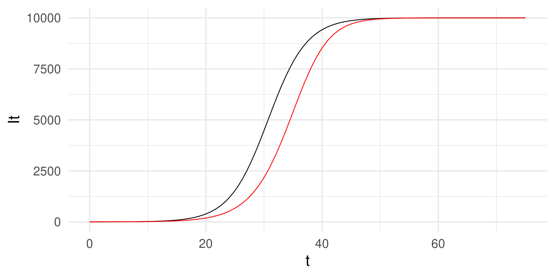
N <-10000I0 <-1dI <-function(I,N,b) b*I*(N - I)/Nbeta <-0.3dt <-1# time increment, # supposed to be infinitesimally smalltmax <-75t <-seq(0,tmax,dt) # this is the vector of timestepsIt <- I0 # this will become the vector # of the number infected I(t) over timefor (i in2:length(t)) { # We iterate over the vector of time steps # and incrementally compute It It[i] = It[i-1] + dt *dI(It[i-1], N, beta) # This is called Euler's method}tibble(t, It) |>ggplot(aes(t,It)) +geom_function( fun =function(t) N / (1+ (N/I0 -1)*exp(-beta*t))) +# Analytical solution for comparisongeom_line(color ="red") +# The numerical solution in blacktheme_minimal(base_size =20)
Why do the graphs deviate? The step size must be “infinitely” small
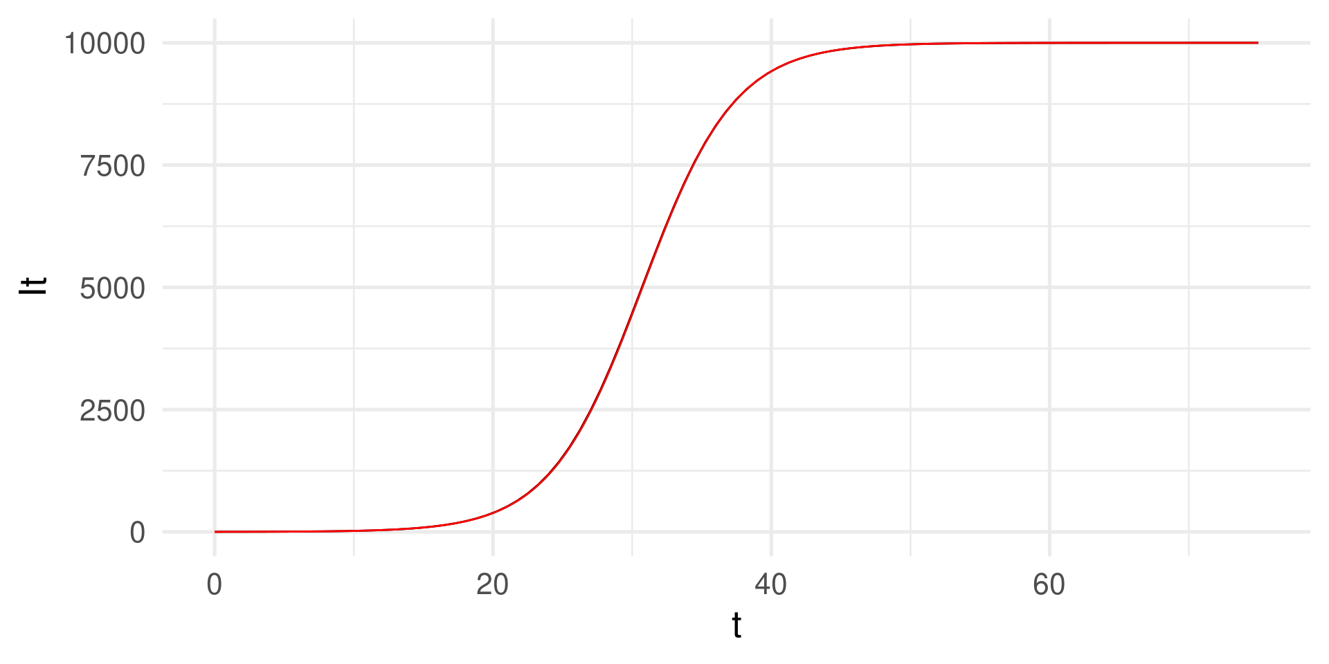
Numerical integration with smaller \(dt\)
We compute the solution step-by-step using small increments of, e.g. \(dt = 0.01\).
N <-10000I0 <-1dI <-function(I,N,b) b*I*(N - I)/Nbeta <-0.3dt <-0.01# time increment, # supposed to be infinitesimally smalltmax <-75t <-seq(0,tmax,dt) # this is the vector of timestepsIt <- I0 # this will become the vector # of the number infected I(t) over timefor (i in2:length(t)) { # We iterate over the vector of time steps # and incrementally compute It It[i] = It[i-1] + dt *dI(It[i-1], N, beta) # This is called Euler's method}tibble(t, It) |>ggplot(aes(t,It)) +geom_function( fun =function(t) N / (1+ (N/I0 -1)*exp(-beta*t))) +# Analytical solution for comparisongeom_line(color ="red") +# The numerical solution in blacktheme_minimal(base_size =20)
Mechanistic model
The SI model is a potential answer to the mechanistic questionHow do epidemics spread?
The examples above show 3 different ways to explore the model:
Agent-based simulation
We model every individual explicitly
Simulation involve random numbers! So simulation runs can be different!
Numerical integration of differential equation
Needs a more abstract concept of compartments
Analytical solutions of differential equation
often not possible (therefore numerical integration is common)
Differentiation with data
We can do calculus operations with data!
In empirical data we can compute the increase in a vector with the function diff:
x <-c(1,2,4,5,5,3,0)diff(x)
[1] 1 2 1 0 -2 -3
More convenient in a data frame is to use x - lag(x) because the vector has the same length.
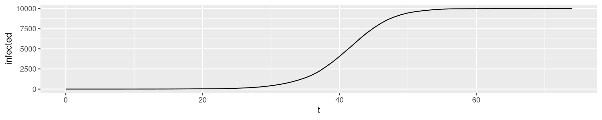
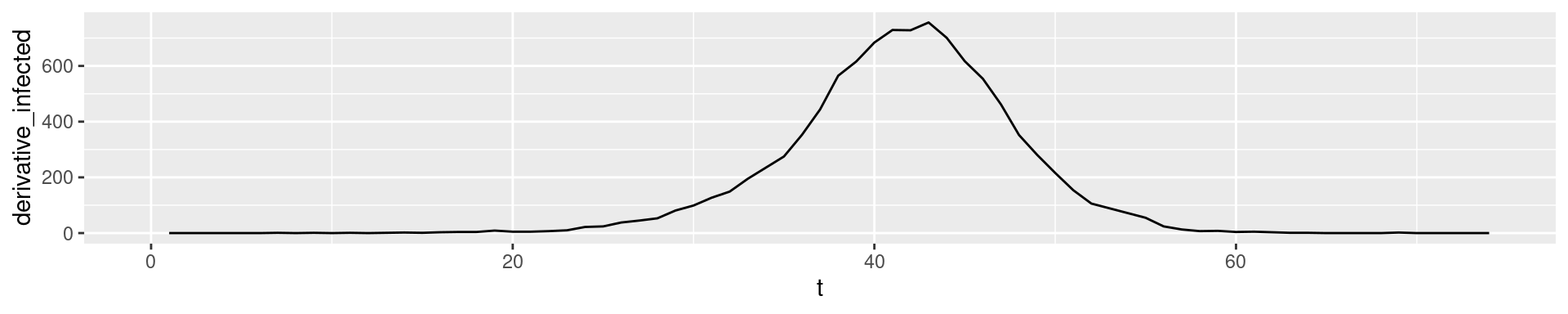
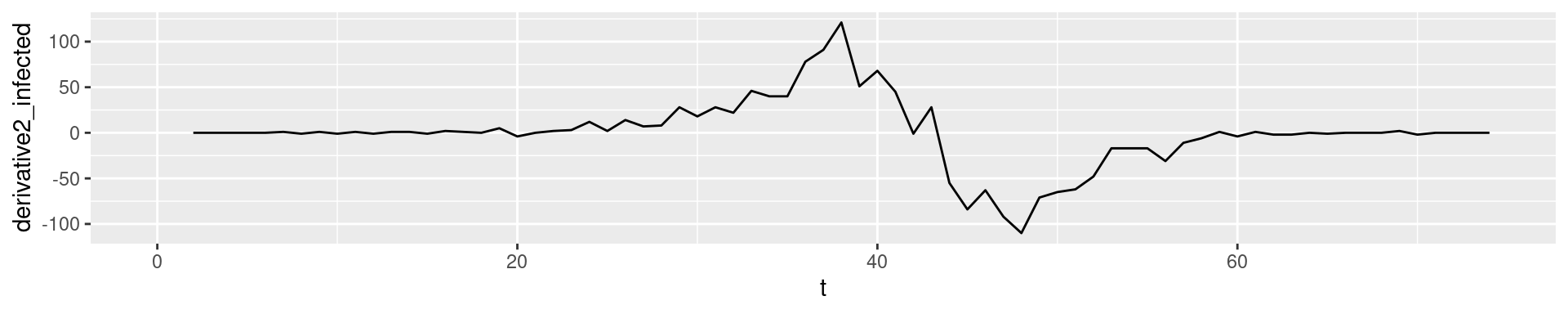
In empirical data: Derivatives of higher order tend to show fluctuation
Interpretation in SI-model
\(I(t)\) total number of infected
\(I'(t)\) number of new cases per day (time step)
\(I''(t)\) how the number of new cases has changes compared to yesterday
2nd derivatives are a good early indicator for the end of a wave.
Integration
The integral of the daily new cases from the beginning to day \(s\) is \(\int_{-\infty}^s f(t)dt\) and represents the total cases at day \(s\).
The integral of a function \(f\) up to time \(s\) is also called the anti-derivative\(F(s) = \int_{-\infty}^s f(t)dt\).
The symbol \(\int\) comes from an S and means “sum”.
Compute the anti-derivative of data vector with cumsum.
x <-c(1,2,4,5,5,3,0)cumsum(x)
[1] 1 3 7 12 17 20 20
Empirically: Derivatives tend to become noisy, while integrals tend to become smooth.
The fundamental theorem of calculus
The integral of the derivative is the function itself.
This is not a proof but shows the idea:
f <-c(1,2,4,5,5,3,0)antiderivative <-cumsum(f)antiderivative
[1] 1 3 7 12 17 20 20
diff(c(0, antiderivative))
[1] 1 2 4 5 5 3 0
# We have to put 0 before to regain the full vectorderivative <-diff(f)derivative
[1] 1 2 1 0 -2 -3
cumsum(c(1,derivative))
[1] 1 2 4 5 5 3 0
# We have to put in the first value (here 1)
# manually because it was lost during the diff
Linear Model
The first work-horse to explore relations between numerical variables
Different purposes of models
Agent-based models and differential equations are usually used to explain the dynamics of one or more variables typically over time. They are used to answer mechanistic questions.
In the following we treat variable-based models which we use to
explain relations between variables
make predictions
These are often used to answer inferential and predictive questions.
(With experimental or more theoretical effort also for causal questions.)
This is a less theory-driven and more data-driven model. Why? We don’t have a simple mathematical form of the function.
Terminology variable-based models
Response variable:1 Variable whose behavior or variation you are trying to understand, on the y-axis
Explanatory variable(s):2 Other variable(s) that you want to use to explain the variation in the response, on the x-axis
Predicted value: Output of the model function.
The model function gives the (expected) average value of the response variable conditioning on the explanatory variables
Residual(s): A measure of how far away a case is from its predicted value (based on the particular model)
Residual = Observed value - Predicted value
The residual tells how far above/below the expected value each case is
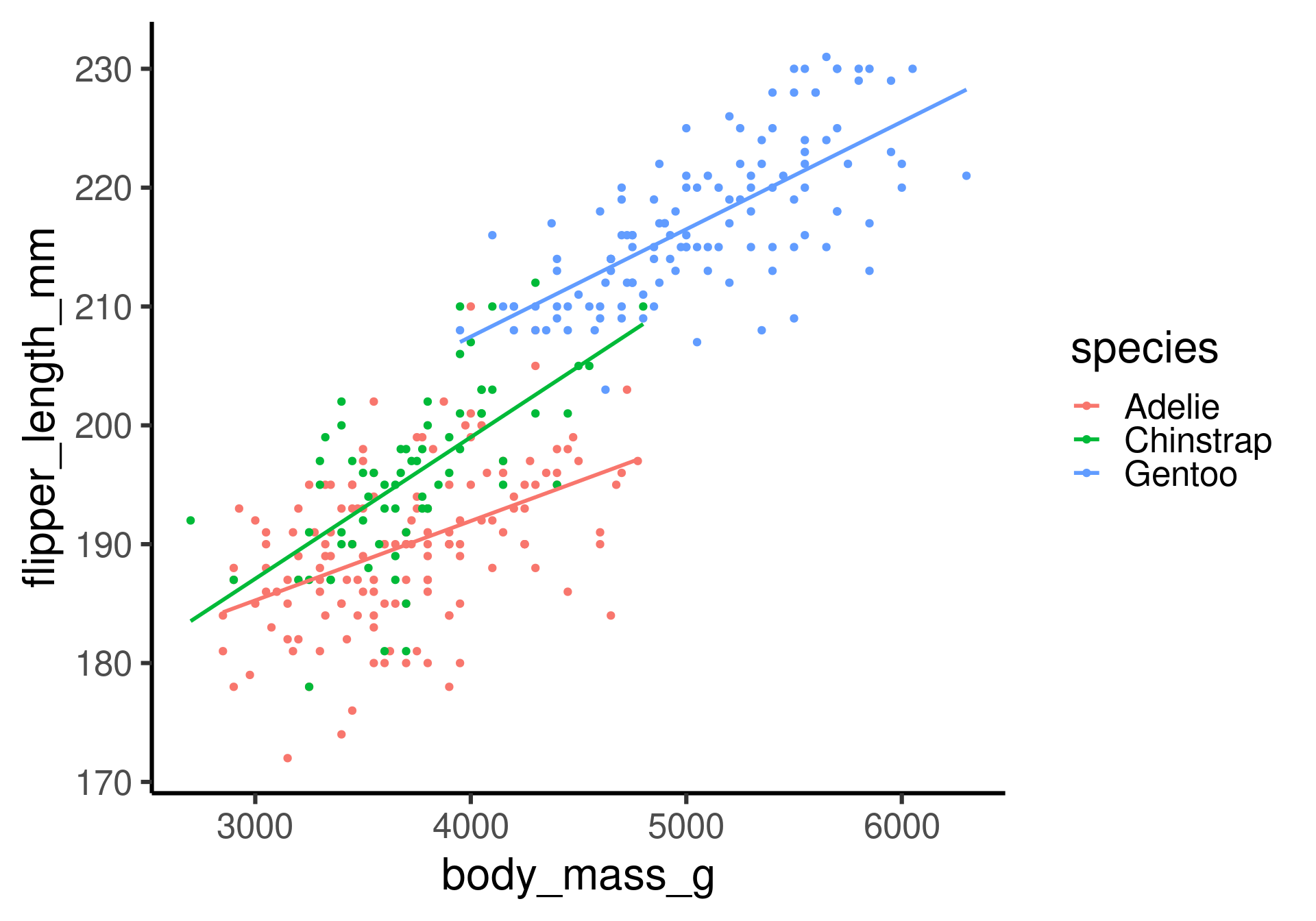
More explanatory variables
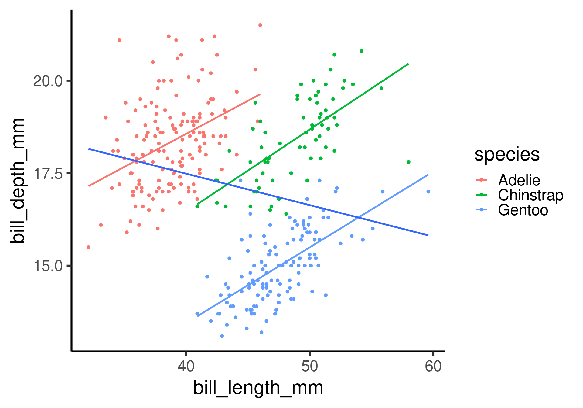
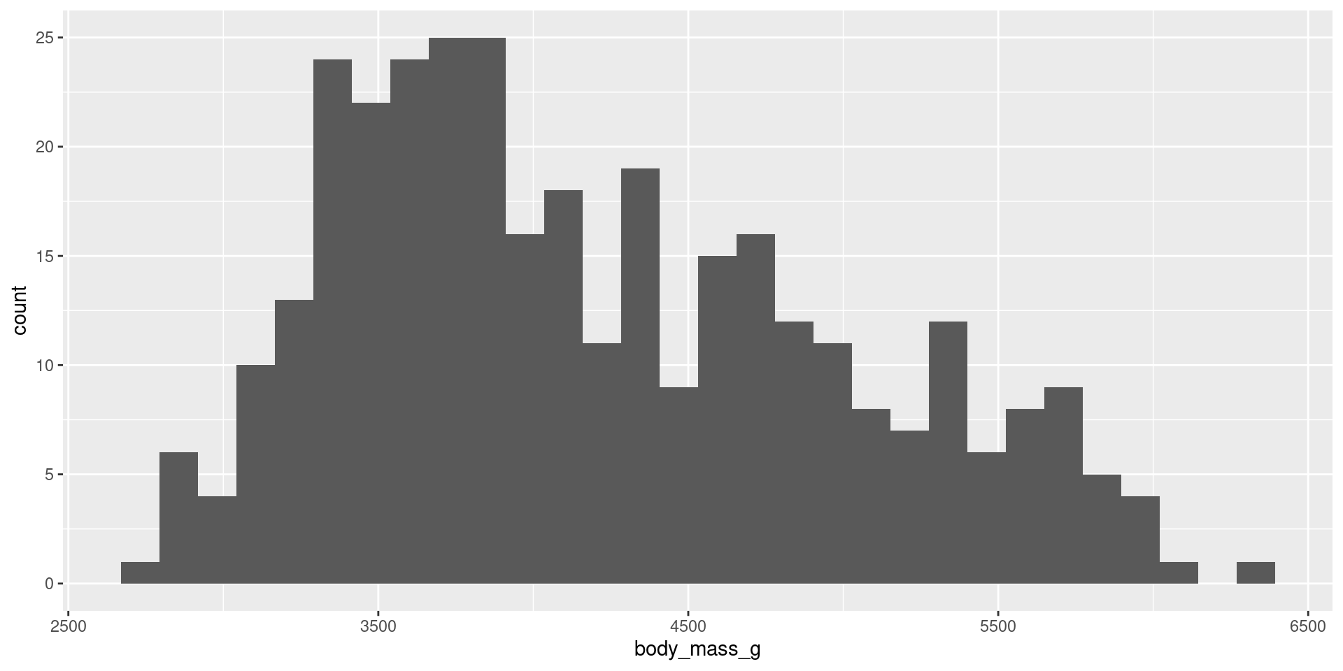
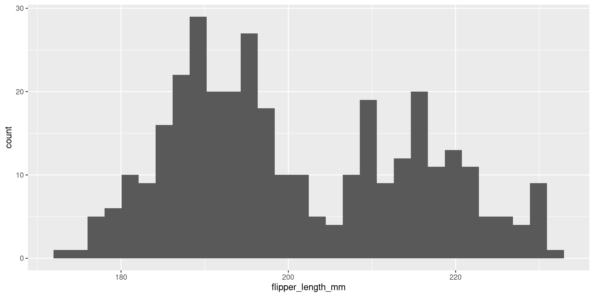
How does the relation between flipper length and body mass change with different species?
penguins |>ggplot(aes(x = body_mass_g, y = flipper_length_mm, color = species)) +geom_point() +geom_smooth(method ="lm",se =FALSE) +theme_classic(base_size =24)
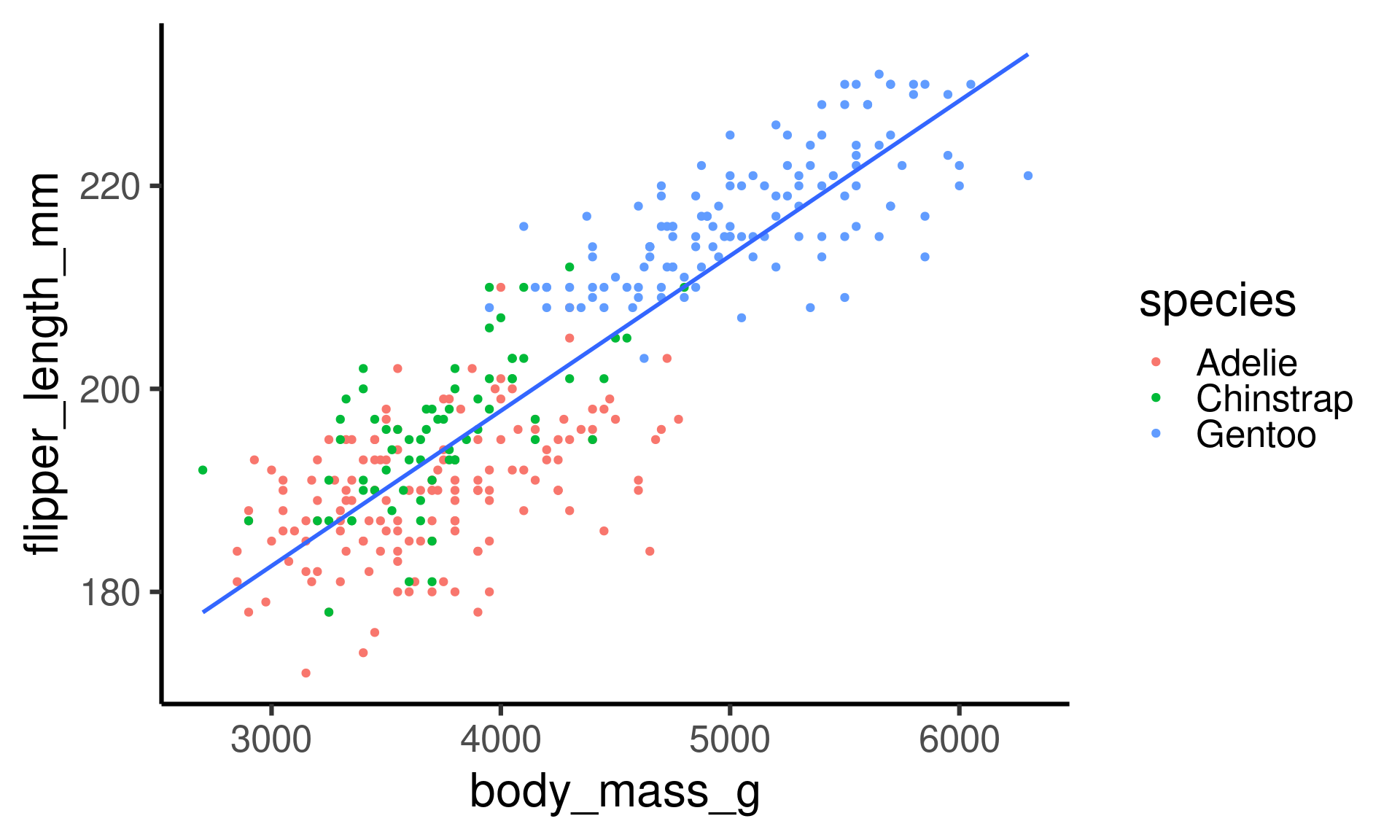
ggplot-hint: How to color penguins but keep one model?
Put the mapping of the color aesthetic into the geom_point command.
penguins |>ggplot(aes(x = body_mass_g, y = flipper_length_mm)) +geom_point(aes(color = species)) +geom_smooth(method ="lm", se =FALSE) +theme_classic(base_size =24)
Beware of Simpson’s paradox
Slopes for all groups can be in the opposite direction of the main effect’s slope!
Models can reveal patterns that are not evident in a graph of the data. This is an advantage of modeling over simple visual inspection of data.
How would you visualize dependencies of more than two variables?
The risk is that a model is imposing structure that is not really there in the real world data.
People imagined animal shapes in the stars. This is maybe a good model to detect and memorize shapes, but it has nothing to do with these animals.
Every model is a simplification of the real world, but there are good and bad models (for particular purposes).
A skeptical (but constructive) approach to a model is always advisable.
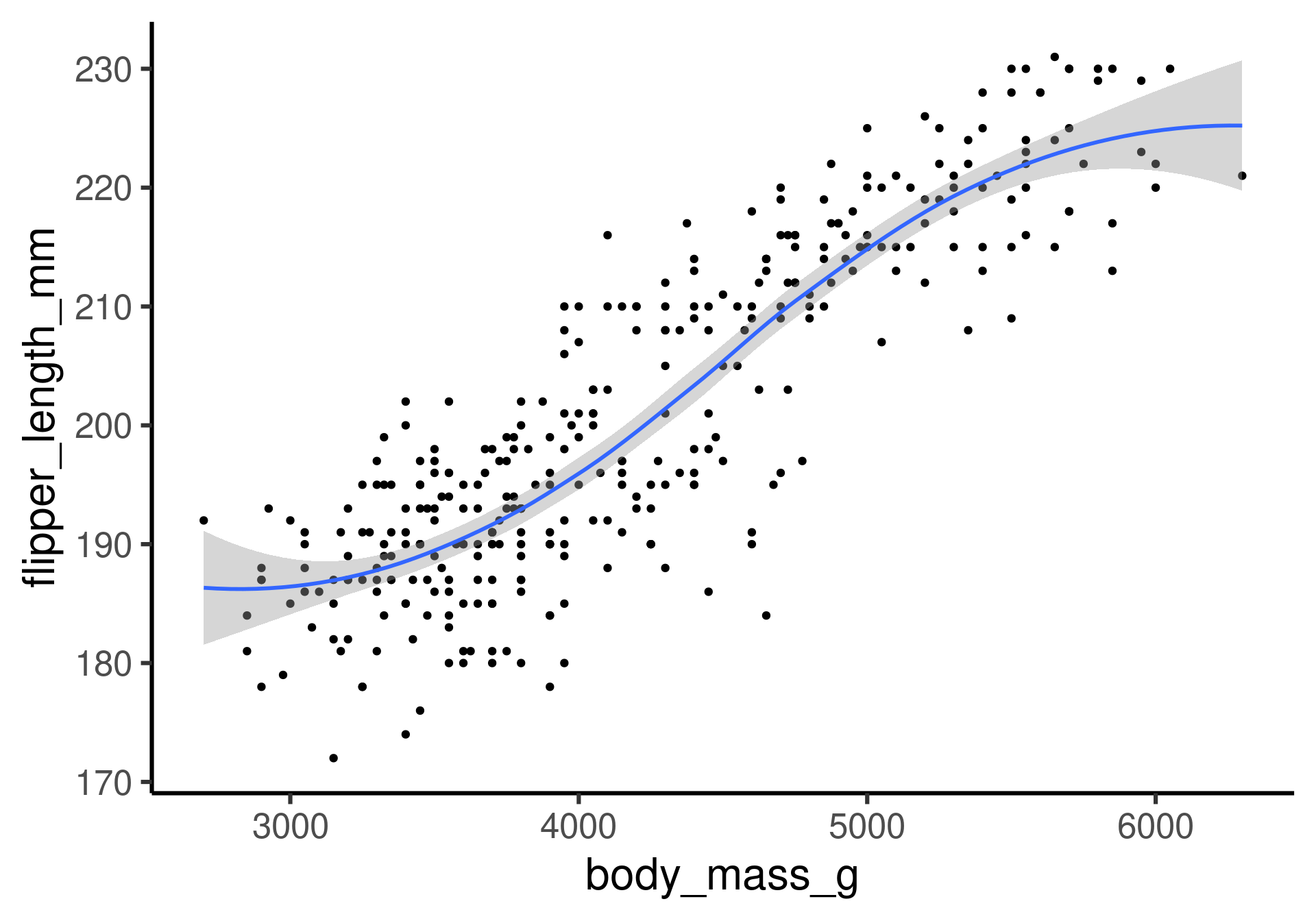
Variation around a model
… is as interesting and important as the model!
Statistics is the explanation of uncertainty of variation in the context of what remains unexplained.
The scattered data of flipper length and body mass suggests that there maybe other factors that account for some parts of the variability.
Or is it randomness?
Adding more explanatory variables can help (but need not)
All models are wrong …
… but some are useful. (George Box)
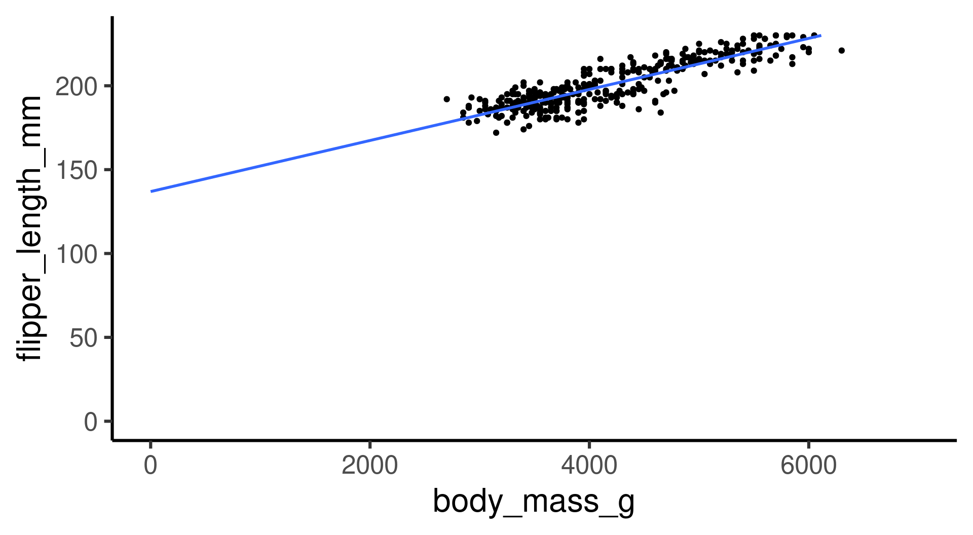
Extending the range of the model:
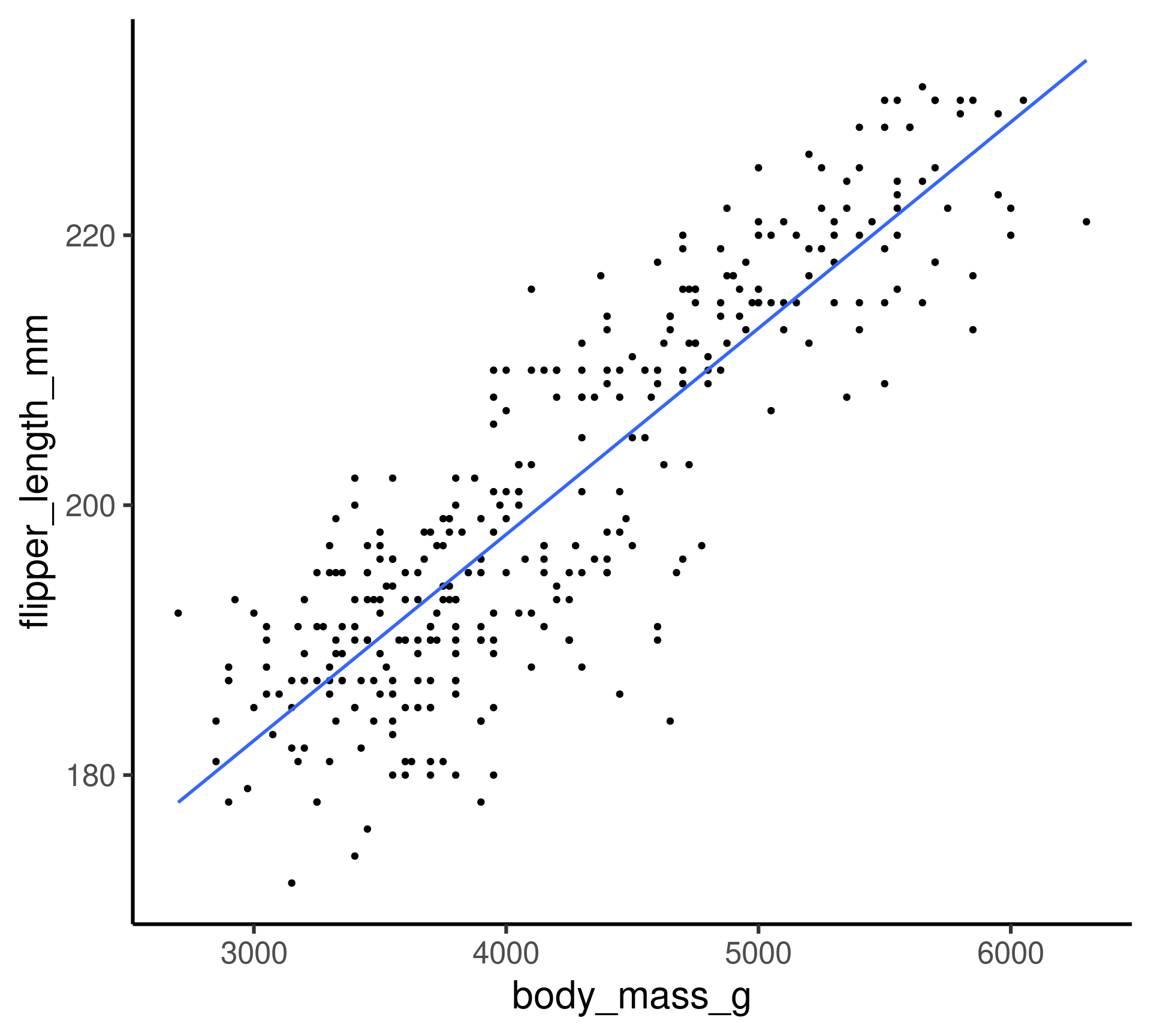
penguins |>ggplot(aes(x = body_mass_g, y = flipper_length_mm)) +geom_point() +geom_smooth(method ="lm", se =FALSE, fullrange =TRUE) +xlim(c(0,7000)) +ylim(c(0,230)) +theme_classic(base_size =24)
The model predicts that penguins with zero weight still have flippers of about 140 mm on average.
Is the model useless? Yes, around zero body mass. No, it works OK in the range of the body mass data.
Two model purposes
Linear models can be used for:
Explanation: Understand the relationship of variables in a quantitative way. For the linear model, interpret slope and intercept.
Prediction: Plug in new values for the explanatory variable(s) and receive the expected response value. For the linear model, predict the flipper length of new penguins by their body mass.
Fitting Models (Part 1)
Today: The linear model.
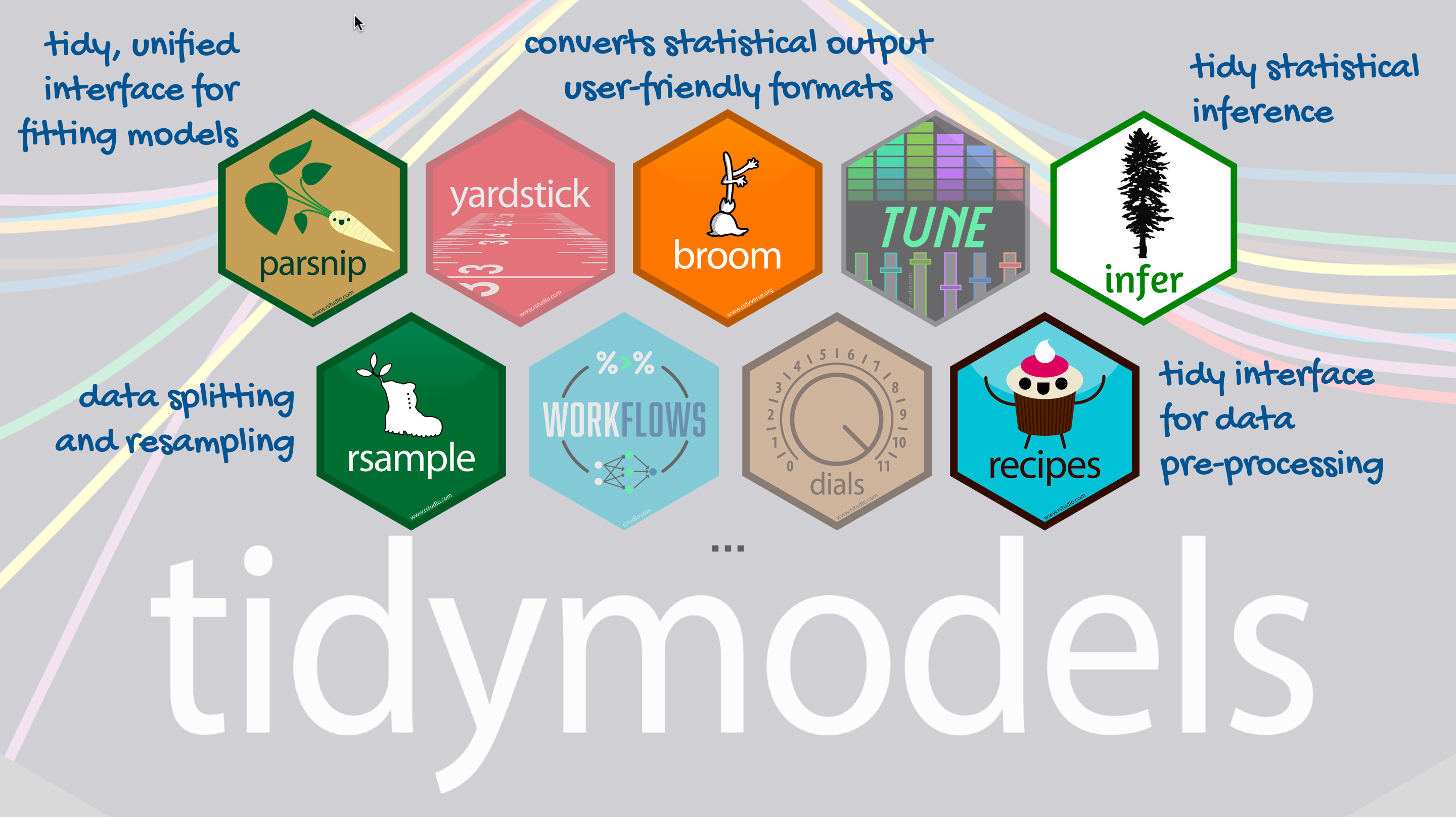
In R: tidymodels
Our goal
Predict flipper length from body mass
average flipper_length_mm\(= \beta_0 + \beta_1\cdot\)body_mass_g
Step 1: Specify model
library(tidymodels)linear_reg()
Linear Regression Model Specification (regression)

Computational engine: lm
Step 2: Set the model fitting engine
linear_reg() |>set_engine("lm")
Linear Regression Model Specification (regression)

Computational engine: lm
Step 3: Fit model and estimate parameters
Only now, the data and the variable selection comes in.
Use of formula syntax
linear_reg() |>set_engine("lm") |>fit(flipper_length_mm ~ body_mass_g, data = penguins)
parsnip model object


Call:
stats::lm(formula = flipper_length_mm ~ body_mass_g, data = data)

Coefficients:
(Intercept)  body_mass_g
  136.72956      0.01528
parsnip is package in tidymodels which is to provide a tidy, unified interface to models that can be used to try a range of models.
What does the output say?
linear_reg() |>set_engine("lm") |>fit(flipper_length_mm ~ body_mass_g, data = penguins)
parsnip model object


Call:
stats::lm(formula = flipper_length_mm ~ body_mass_g, data = data)

Coefficients:
(Intercept)  body_mass_g
  136.72956      0.01528
average flipper_length_mm\(= 136.72956 + 0.01528\cdot\)body_mass_g
Interpretation:
The penguins have a flipper length of 138 mm plus 0.01528 mm for each gram of body mass (that is 15.28 mm per kg). Penguins with zero mass have a flipper length of 138 mm. However, this is not in the range where the model was fitted.
Show output in tidy form
linear_reg() |>set_engine("lm") |>fit(flipper_length_mm ~ body_mass_g, data = penguins) |>tidy()
Notation from statistics: \(\beta\)’s for the population parameters and \(\hat\beta\)’s for the parameters estimated from the sample statistics.
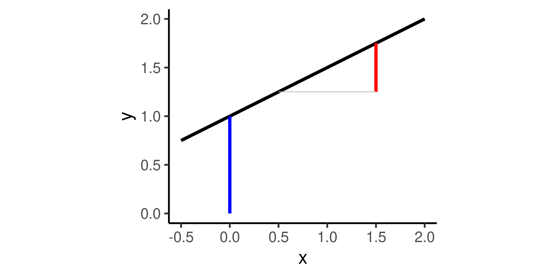
\[\hat y = \beta_0 + \beta_1 x\]
Is what we cannot have. (\(\hat y\) stands for predicted value of \(y\). )
We estimate \(\hat\beta_0\) and \(\hat\beta_1\) in the model fitting process.
\[\hat y = \hat\beta_0 + \hat\beta_1 x\]
A typical follow-up data analysis question is what the fitted values \(\hat\beta_0\) and \(\hat\beta_1\) tell us about the population-wide values \(\beta_0\) and \(\beta_1\)?


 ::: aside Source: https://upload.wikimedia.org/wikipedia/commons/f/fb/Simpsons_paradox_-_animation.gif :::