W#05: Summary Statistics, Exploratory Data Analysis, Principal Component Analysis

Jan Lorenz

Summary Statistics (continued)

Data Sets 1a and 1b: Widsom of Crowd

1a: Ox weigh guessing competition 1907 (collected by Galton)

galton |> ggplot(aes(Estimate)) + geom_histogram(binwidth = 5)

1b: Viertelfest “guess the number of sold lots”-competition 2009

viertel |> filter(Schätzung<100000) |> ggplot(aes(`Schätzung`)) + geom_histogram(binwidth = 500)

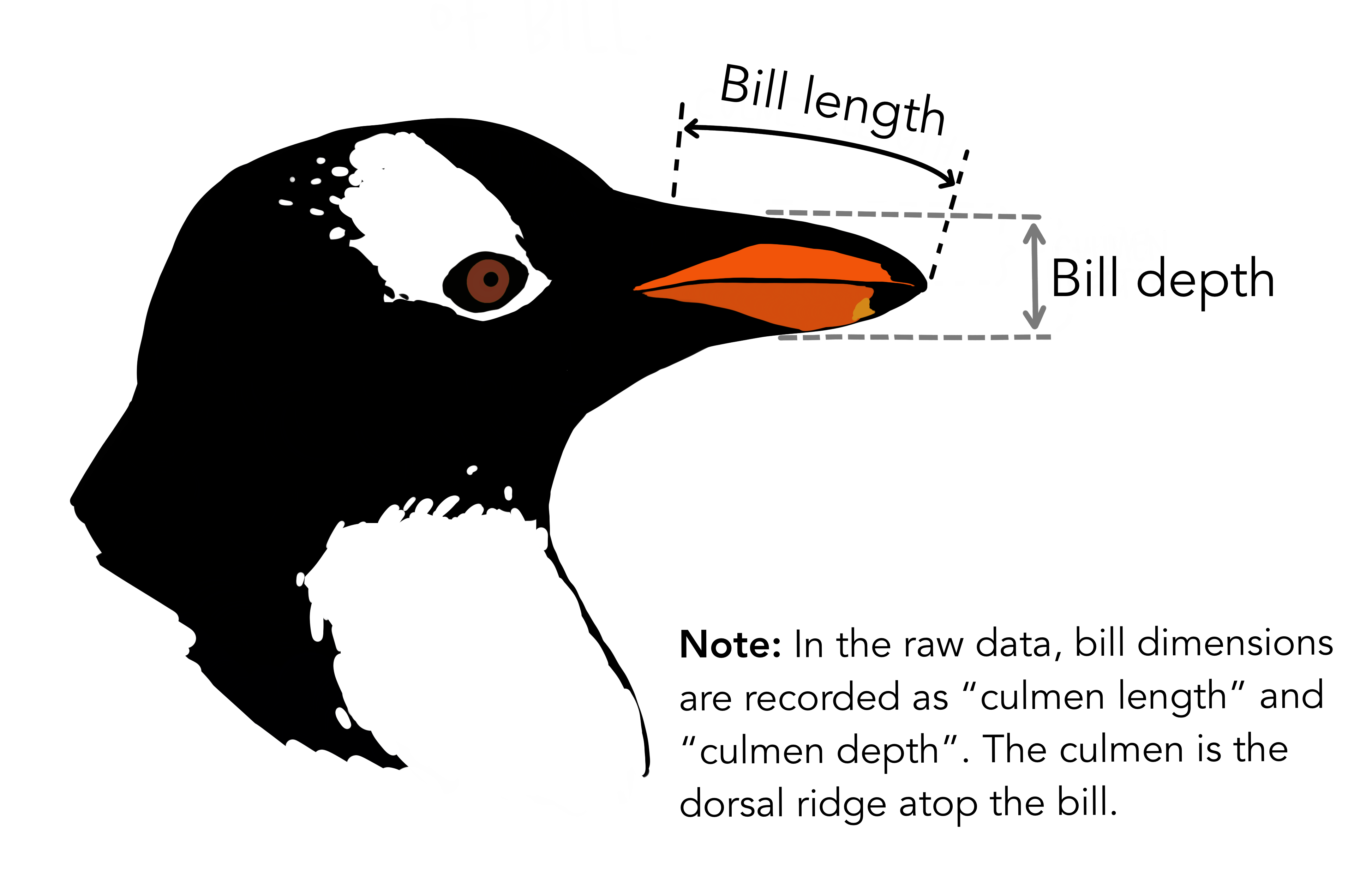
Data Set 2: Palmer Penguins

Palmer Penguins

Chinstrap, Gentoo, and Adélie Penguins

# A tibble: 344 × 8
   species island    bill_length_mm bill_depth_mm flipper_length_mm body_mass_g
   <fct>   <fct>              <dbl>         <dbl>             <int>       <int>
 1 Adelie  Torgersen           39.1          18.7               181        3750
 2 Adelie  Torgersen           39.5          17.4               186        3800
 3 Adelie  Torgersen           40.3          18                 195        3250
 4 Adelie  Torgersen           NA            NA                  NA          NA
 5 Adelie  Torgersen           36.7          19.3               193        3450
 6 Adelie  Torgersen           39.3          20.6               190        3650
 7 Adelie  Torgersen           38.9          17.8               181        3625
 8 Adelie  Torgersen           39.2          19.6               195        4675
 9 Adelie  Torgersen           34.1          18.1               193        3475
10 Adelie  Torgersen           42            20.2               190        4250
# ℹ 334 more rows
# ℹ 2 more variables: sex <fct>, year <int>

summary from base R

Shows summary statistics for the values in a vector

summary(galton$Estimate)

   Min. 1st Qu.  Median    Mean 3rd Qu.    Max. 
    896    1162    1208    1197    1236    1516 

summary(viertel$Schätzung)

    Min.  1st Qu.   Median     Mean  3rd Qu.     Max. 
     120     5000     9843    53164    20000 29530000 

Or for all columns in a data frame

summary(penguins)

      species          island    bill_length_mm  bill_depth_mm  
 Adelie   :152   Biscoe   :168   Min.   :32.10   Min.   :13.10  
 Chinstrap: 68   Dream    :124   1st Qu.:39.23   1st Qu.:15.60  
 Gentoo   :124   Torgersen: 52   Median :44.45   Median :17.30  
                                 Mean   :43.92   Mean   :17.15  
                                 3rd Qu.:48.50   3rd Qu.:18.70  
                                 Max.   :59.60   Max.   :21.50  
                                 NA's   :2       NA's   :2      
 flipper_length_mm  body_mass_g       sex           year     
 Min.   :172.0     Min.   :2700   female:165   Min.   :2007  
 1st Qu.:190.0     1st Qu.:3550   male  :168   1st Qu.:2007  
 Median :197.0     Median :4050   NA's  : 11   Median :2008  
 Mean   :200.9     Mean   :4202                Mean   :2008  
 3rd Qu.:213.0     3rd Qu.:4750                3rd Qu.:2009  
 Max.   :231.0     Max.   :6300                Max.   :2009  
 NA's   :2         NA's   :2                                 

Question

What does
1st Qu. and
3rd Qu. mean?

Quantiles

Cut points specifying intervals which contain equal amounts of values of the distribution.

\(q\)-quantiles divide numbers into \(q\) intervals covering all values.

The quantiles are the cut points: For \(q\) intervals there are \(q-1\) cut points of interest.

• The one 2-quantile is the median
• The three 4-quantiles are called quartiles
  • 1st Qu. is the first quartile
  • The second quartile is the median
  • 3rd Qu. is the third quartile
• 100-quantiles are called percentiles

We omit problems of estimating quantiles from a sample where the number of estimates does not fit to a desired partition of equal size here.

1a Galton: Quartiles

# Min, 3 Quartiles, Max
quantile(galton$Estimate, prob = seq(0, 1, by = 0.25))

    0%    25%    50%    75%   100% 
 896.0 1162.5 1208.0 1236.0 1516.0 

Interpretation: What does the value at 25% mean?

The 25% of all values are lower than the value. 75% are larger.

galton |> ggplot(aes(Estimate)) + geom_histogram(binwidth = 5) + 
 geom_vline(xintercept = quantile(galton$Estimate, prob = seq(0, 1, by = 0.25)), color = "red")

1a Galton: 20-quantiles

# Min, 3 Quartiles, Max
quantile(galton$Estimate, prob = seq(0, 1, by = 0.05))

    0%     5%    10%    15%    20%    25%    30%    35%    40%    45%    50% 
 896.0 1078.3 1109.0 1126.9 1150.0 1162.5 1174.0 1181.0 1189.0 1199.0 1208.0 
   55%    60%    65%    70%    75%    80%    85%    90%    95%   100% 
1214.0 1219.0 1225.0 1231.0 1236.0 1243.8 1255.1 1270.0 1293.0 1516.0 

galton |> ggplot(aes(Estimate)) + geom_histogram(binwidth = 5) + 
 geom_vline(xintercept = quantile(galton$Estimate, prob = seq(0, 1, by = 0.05)), color = "red")

1b Viertelfest: Quartiles

quantile(viertel$Schätzung, prob = seq(0, 1, by = 0.25))

      0%      25%      50%      75%     100% 
     120     5000     9843    20000 29530000 

viertel |> filter(Schätzung<100000) |> ggplot(aes(`Schätzung`)) + geom_histogram(binwidth = 500) + 
 geom_vline(xintercept = quantile(viertel$`Schätzung`, prob = seq(0, 1, by = 0.25))[1:4], color = "red")

1b Viertelfest: 20-quantiles

quantile(viertel$Schätzung, prob = seq(0, 1, by = 0.05))

         0%          5%         10%         15%         20%         25% 
     120.00     1213.25     2000.00     3115.00     4012.00     5000.00 
        30%         35%         40%         45%         50%         55% 
    5853.50     7000.00     7821.00     8705.25     9843.00    10967.50 
        60%         65%         70%         75%         80%         85% 
   12374.00    14444.00    16186.00    20000.00    27500.00    38000.00 
        90%         95%        100% 
   63649.50    99773.50 29530000.00 

viertel |> filter(Schätzung<100000) |> ggplot(aes(`Schätzung`)) + geom_histogram(binwidth = 500) + 
 geom_vline(xintercept = quantile(viertel$`Schätzung`, prob = seq(0, 1, by = 0.05))[1:19], color = "red")

2 Palmer Penguins Flipper Length: Quartiles

quantile(penguins$flipper_length_mm, prob = seq(0, 1, by = 0.25), na.rm = TRUE)

  0%  25%  50%  75% 100% 
 172  190  197  213  231 

penguins |> ggplot(aes(flipper_length_mm)) + geom_histogram(binwidth = 1) + 
 geom_vline(xintercept = quantile(penguins$flipper_length_mm, prob = seq(0, 1, by = 0.25), na.rm = TRUE), color = "red")

2 Palmer Penguins Flipper Length: 20-quantiles

quantile(penguins$flipper_length_mm, prob = seq(0, 1, by = 0.05), na.rm = TRUE)

   0%    5%   10%   15%   20%   25%   30%   35%   40%   45%   50%   55%   60% 
172.0 181.0 185.0 187.0 188.0 190.0 191.0 193.0 194.0 195.0 197.0 199.0 203.0 
  65%   70%   75%   80%   85%   90%   95%  100% 
208.0 210.0 213.0 215.0 218.0 220.9 225.0 231.0 

penguins |> ggplot(aes(flipper_length_mm)) + geom_histogram(binwidth = 1) + 
 geom_vline(xintercept = quantile(penguins$flipper_length_mm, prob = seq(0, 1, by = 0.05), na.rm = TRUE), color = "red")

Interquartile range (IQR)

The difference between the 1st and the 3rd quartile. Alternative dispersion measure.
The range in which the middle 50% of the values are located.

Examples:

# Min, 3 Quartiles, Max
IQR(galton$Estimate)

[1] 73.5

sd(galton$Estimate) # for comparison

[1] 73.58677

IQR(viertel$Schätzung)

[1] 15000

sd(viertel$Schätzung) # for comparison

[1] 848395.5

IQR(penguins$flipper_length_mm, na.rm = TRUE)

[1] 23

sd(penguins$flipper_length_mm, na.rm = TRUE) # for comparison

[1] 14.06171

Boxplots

A condensed visualization of a distribution showing location, spread, skewness and outliers.

galton |> ggplot(aes(x = Estimate)) + geom_boxplot()

• The box shows the median in the middle and the other two quartiles as their borders.
• Whiskers: From above the upper quartile, a distance of 1.5 times the IQR is measured out and a whisker is drawn up to the largest observed data point from the dataset that falls within this distance. Similarly, for the lower quartile.
• Whiskers must end at an observed data point! (So lengths can differ.)
• All other values outside of box and whiskers are shown as points and often called outliers. (There may be none.)

Boxplots vs. histograms

• Histograms can show the shape of the distribution well, but not the summary statistics like the median.

galton |> ggplot(aes(x = Estimate)) + geom_boxplot()

galton |> ggplot(aes(x = Estimate)) + geom_histogram(binwidth = 5)

Boxplots vs. histograms

• Boxplots can not show the patterns of bimodal or multimodal distributions.

palmerpenguins::penguins |> ggplot(aes(x = flipper_length_mm)) + geom_boxplot()

palmerpenguins::penguins |> ggplot(aes(x = flipper_length_mm)) + geom_histogram(binwidth = 1)

Minimizing proporties of Mean and Median

Mean minimizes the mean of squared deviations from it. No other value \(a\) has a lower mean of square distances from the data points. \(\frac{1}{n}\sum_{i=1}^n(x_i - a)^2\).

Median minimizes the sum of the absolute deviation. No other value \(a\) has a lower mean of absolute distances from the data points. \(\frac{1}{n}\sum_{i=1}^n|x_i - a|\).

Two families of summary statistics

• Measures based on sums (related to mathematical moments)
  • Mean
  • Standard deviation
• Measures based on the ordered sequence of these observations (order statistics)
  • Median (and all quantiles)
  • Interquartile range

Bivariate Summary Statistics

Covariance

Goal: We want to measure the joint variation in numerical observations of two variables \(x_1,\dots,x_n\) and \(y_1, \dots, y_n\).

Covariance

\(\text{cov}(x,y) = \frac{1}{n}\sum_{i=1}^n(x_i - \mu_x)(y_i - \mu_y)\)

where \(\mu_x\) and \(\mu_y\) are the arithmetic means of \(x\) and \(y\).

Note: \(\text{cov}(x,x) = \frac{1}{n}\sum_{i=1}^n(x_i - \mu_x)(x_i - \mu_x) = \frac{1}{n}\sum_{i=1}^n(x_i - \mu_x)^2 = \text{Var}(x)\)

Correlation

Goal: We want to measure the linear correlation in numerical observations of two variables \(x_1,\dots,x_n\) and \(y_1, \dots, y_n\).

Pearson correlation coefficient \(r_{xy} = \frac{\sum_{i=1}^n(x_i - \mu_x)(y_i - \mu_y)}{\sqrt{\sum_{i=1}^n(x_i - \mu_x)^2}\sqrt{\sum_{i=1}^n(y_i - \mu_y)^2}}\)

Relation to covariance: \(r_{xy} = \frac{\text{cov}(x,y)}{\sigma_x\sigma_y}\)

where \(\sigma_x\) and \(\sigma_y\) are the standard deviations of \(x\) and \(y\).

Relation to standard scores:
When \(x\) and \(y\) are standard scores (each with mean zero and standard deviation one), then \(\text{cov}(x,y) = r_{xy}\).

There are other correlation coefficients which we omit here.

Interpretation of correlation

Correlation between two vectors \(x\) and \(y\) is “normalized”.

• The maximal possible values is \(r_{xy} = 1\)
  • \(x\) and \(y\) are fully correlated
• The minimal values is \(r_{xy} = -1\)
  • \(x\) and \(y\) are anticorrelated
• \(r_{xy} \approx 0\) mean
  • the variables are uncorrelated
• \(r_{xy} = r_{yx}\)

Correlation matrix

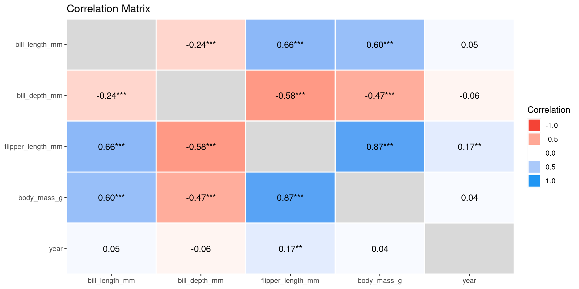
Using corrr from the packagestidymodels

library(corrr)
penguins |> select(-species, -island, -sex) |> 
 correlate()

# A tibble: 5 × 6
  term        bill_length_mm bill_depth_mm flipper_length_mm body_mass_g    year
  <chr>                <dbl>         <dbl>             <dbl>       <dbl>   <dbl>
1 bill_lengt…        NA            -0.235              0.656      0.595   0.0545
2 bill_depth…        -0.235        NA                 -0.584     -0.472  -0.0604
3 flipper_le…         0.656        -0.584             NA          0.871   0.170 
4 body_mass_g         0.595        -0.472              0.871     NA       0.0422
5 year                0.0545       -0.0604             0.170      0.0422 NA     

Correlation table

Using correlation from the packagescorrelation

library(correlation)
results <- palmerpenguins::penguins |> 
 select(-species, -island, -sex) |> 
 correlation()
results

# Correlation Matrix (pearson-method)

Parameter1        |        Parameter2 |     r |         95% CI | t(340) |         p
-----------------------------------------------------------------------------------
bill_length_mm    |     bill_depth_mm | -0.24 | [-0.33, -0.13] |  -4.46 | < .001***
bill_length_mm    | flipper_length_mm |  0.66 | [ 0.59,  0.71] |  16.03 | < .001***
bill_length_mm    |       body_mass_g |  0.60 | [ 0.52,  0.66] |  13.65 | < .001***
bill_length_mm    |              year |  0.05 | [-0.05,  0.16] |   1.01 | 0.797    
bill_depth_mm     | flipper_length_mm | -0.58 | [-0.65, -0.51] | -13.26 | < .001***
bill_depth_mm     |       body_mass_g | -0.47 | [-0.55, -0.39] |  -9.87 | < .001***
bill_depth_mm     |              year | -0.06 | [-0.17,  0.05] |  -1.11 | 0.797    
flipper_length_mm |       body_mass_g |  0.87 | [ 0.84,  0.89] |  32.72 | < .001***
flipper_length_mm |              year |  0.17 | [ 0.06,  0.27] |   3.17 | 0.007**  
body_mass_g       |              year |  0.04 | [-0.06,  0.15] |   0.78 | 0.797    

p-value adjustment method: Holm (1979)
Observations: 342

What do the stars mean? Statistical significance automatically added by the . We treat that later.

Correlation visualization

results %>%
  summary(redundant = TRUE) %>%
  plot()

Exploratory Data Analysis

Exploratory Data Analysis

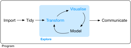
EDA is the systematic exploration of data using

• visualization
• transformation
• computation of characteristic values
• modeling

Computation of characteristic values: Functions like mean, median, mode, standard deviation, or interquartile range
Modeling: Operations like linear regression or dimensionality reduction. We haven’t talked about it, but will do soon.

Systematic but no standard routine

“There are no routine statistical questions, only questionable statistical routines.” — Sir David Cox

“Far better an approximate answer to the right question, which is often vague, than an exact answer to the wrong question, which can always be made precise.” — John Tukey

Systematic but no standard routine

• Goal of EDA: Develop understanding of your data.
• EDA’s iterative cycle
  1. Generate questions about your data.
  2. Search for answers by visualizing, transforming, and modelling your data.
  3. Use what you learn to refine your questions and/or generate new questions.
• EDA is fundamentally a creative process.

Questions

• The way to ask quality questions:
  • Generate many questions!
  • You cannot come up with most interesting questions when you start.
• There is no rule which questions to ask. These are useful
  1. What type of variation occurs within my variables?
     (Barplots, Histograms,…)
  2. What type of covariation occurs between my variables?
     (Scatterplots, Timelines,…)

EDA embedded in a statistical data science project

1. Stating and refining the question
2. Exploring the data
3. Building formal statistical models
4. Interpreting the results
5. Communicating the results

Roger D. Peng and Elizabeth Matsui. “The Art of Data Science.” A Guide for Anyone Who Works with Data. Skybrude Consulting, LLC (2015).

Example EDA: Strange Airports

From Homework 02:

library(nycflights13)
ggplot(data = airports, mapping = aes(x = lon, y = lat)) + geom_point(aes(color = tzone)) 

airports %>% filter(lon >= 0) 

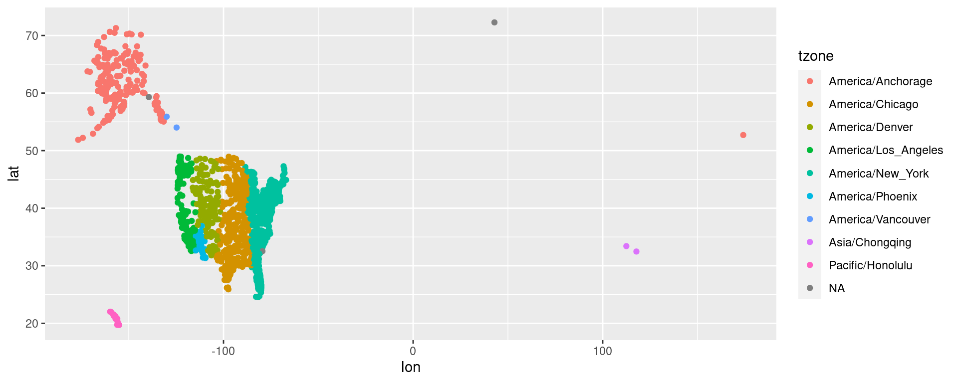
# A tibble: 4 × 8
  faa   name                            lat   lon   alt    tz dst   tzone       
  <chr> <chr>                         <dbl> <dbl> <dbl> <dbl> <chr> <chr>       
1 DVT   Deer Valley Municipal Airport  33.4 112.   1478     8 A     Asia/Chongq…
2 EEN   Dillant Hopkins Airport        72.3  42.9   149    -5 A     <NA>        
3 MYF   Montgomery Field               32.5 118.     17     8 A     Asia/Chongq…
4 SYA   Eareckson As                   52.7 174.     98    -9 A     America/Anc…

Airport errors

# A tibble: 4 × 8
  faa   name                            lat   lon   alt    tz dst   tzone       
  <chr> <chr>                         <dbl> <dbl> <dbl> <dbl> <chr> <chr>       
1 DVT   Deer Valley Municipal Airport  33.4 112.   1478     8 A     Asia/Chongq…
2 EEN   Dillant Hopkins Airport        72.3  42.9   149    -5 A     <NA>        
3 MYF   Montgomery Field               32.5 118.     17     8 A     Asia/Chongq…
4 SYA   Eareckson As                   52.7 174.     98    -9 A     America/Anc…

Correct locations (internet research and location of maps):

• Deer Valley Municipal Airport: Phoenix
  33°41′N 112°05′W Missing minus for lon (W)
• Dillant Hopkins Airport: New Hampshire
  42°54′N 72°16′W lon-lat switched, minus (W)
• Montgomery Field: San Diego
  32°44′N 117°11″W Missing minus for lon (W)
• Eareckson As: Alaska
  52°42′N 174°06′E No error: Too west,it’s east!

Conclusions on data errors

• In real-world datasets errors like the 3 airport are quite common.
• Errors of this type are often hard to detect and remain unnoticed.
  • This can (but need not) change results drastically!

Conclusions

• Always remain alert for inconsistencies and be ready to check the plausibility of results.
• Skills in exploratory data analysis (EDA) are essential to find errors and explore their nature and implication
• Errors are unpredictable, of diverse types, and are often deeply related to the reality the data presents.
  • This is one reason why EDA can not be a fully formalized and automatized process.

Data science projects

Outline of question-driven data work

Six types of questions

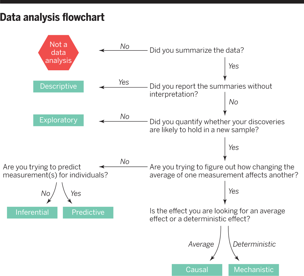
1. Descriptive: summarize a characteristic of a set of data
2. Exploratory: analyze to see if there are patterns, trends, or relationships between variables (hypothesis generating)
3. Inferential: analyze patterns, trends, or relationships in representative data from a population
4. Predictive: make predictions for individuals or groups of individuals
5. Causal: whether changing one factor will change another factor, on average, in a population
6. Mechanistic: explore “how” one factor (probably/most likely/potentially) changes another

We only did 1 and 2, so far.

Leek, Jeffery T., and Roger D. Peng. 2015. “What Is the Question?” Science 347 (6228): 1314–15. https://doi.org/10.1126/science.aaa6146.

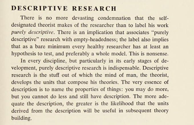
Descriptive Projects

Dubin (1969). Theory Building - A Practical Guide to the Construction and Testing of Theoretical Models

Data Analysis Flowchart

Example: COVID-19 and Vitamin D

1. Descriptive: frequency of hospitalisations due to COVID-19 in a set of data collected from a group of individuals
2. Exploratory: examine relationships between a range of dietary factors and COVID-19 hospitalisations
3. Inferential: examine whether any relationship between taking Vitamin D supplements and COVID-19 hospitalisations found in the sample hold for the population at large
4. Predictive: what types of people will take Vitamin D supplements during the next year
5. Causal: whether people with COVID-19 who were randomly assigned to take Vitamin D supplements or those who were not are hospitalised
6. Mechanistic: how increased vitamin D intake leads to a reduction in the number of viral illnesses

Questions to questions

• Do you have appropriate data to answer your question?
• Do you have information on confounding variables?
• Was the data you’re working with collected in a way that introduces bias?

Example
I want to estimate the average number of children in households in Bremen. I conduct a survey at an elementary school and ask pupils how many children, including themselves, live in their house. Then, I take the average of the responses.

• Is this a biased or an unbiased estimate of the number of children in households in Bremen?
• If biased, will the value be an overestimate or underestimate?

Context Information is important!

• Not all information is in the data!
• Potential confounding variables you infer from general knowledge
• Information about data collection you may receive from an accompanying report
• Information about computed variables you may need to look up in accompanying documentation
• Information about certain variables you may find in an accompanying codebook. For example the exact wording of questions in survey data.

Data Science Projects in the Course

• A project report is the main assessment for the Data Science Tools module.
• This week more homework repositories will be released.
• These homework repositories may be updated with new tasks once new concepts have been treated.
• Topics will for example be
  • COVID-19
  • Germany’s income distribution and income tax
  • Fuel prices in Western Australia
  • Political Attitudes in Germany
  • …
• The repositories mimick data science projects. Later you will choose a data science project on your own. It can build on these topics or on different datasets which you find interesting.

Principal component analysis (PCA)

A typical part of Exploratory Data Analysis.

PCA Description

Principle component analysis

• is a dimensionality-reduction technique, that means it can be used to reduce the number of variables
• computes new variables which represent the data in a different way
• transforms the data linearly to a new coordinate system where most of the variation in the data can be described with fewer variables than the original data

Today: Quick walk through how to use and interpret it.

Example: Numerical variables of penguins

peng <- 
 penguins |> 
 select(species, bill_length_mm, bill_depth_mm, flipper_length_mm, body_mass_g) |> 
 na.omit()
peng |> count(species)

# A tibble: 3 × 2
  species       n
  <fct>     <int>
1 Adelie      151
2 Chinstrap    68
3 Gentoo      123

We have 342 penguins and 4 numeric variables.

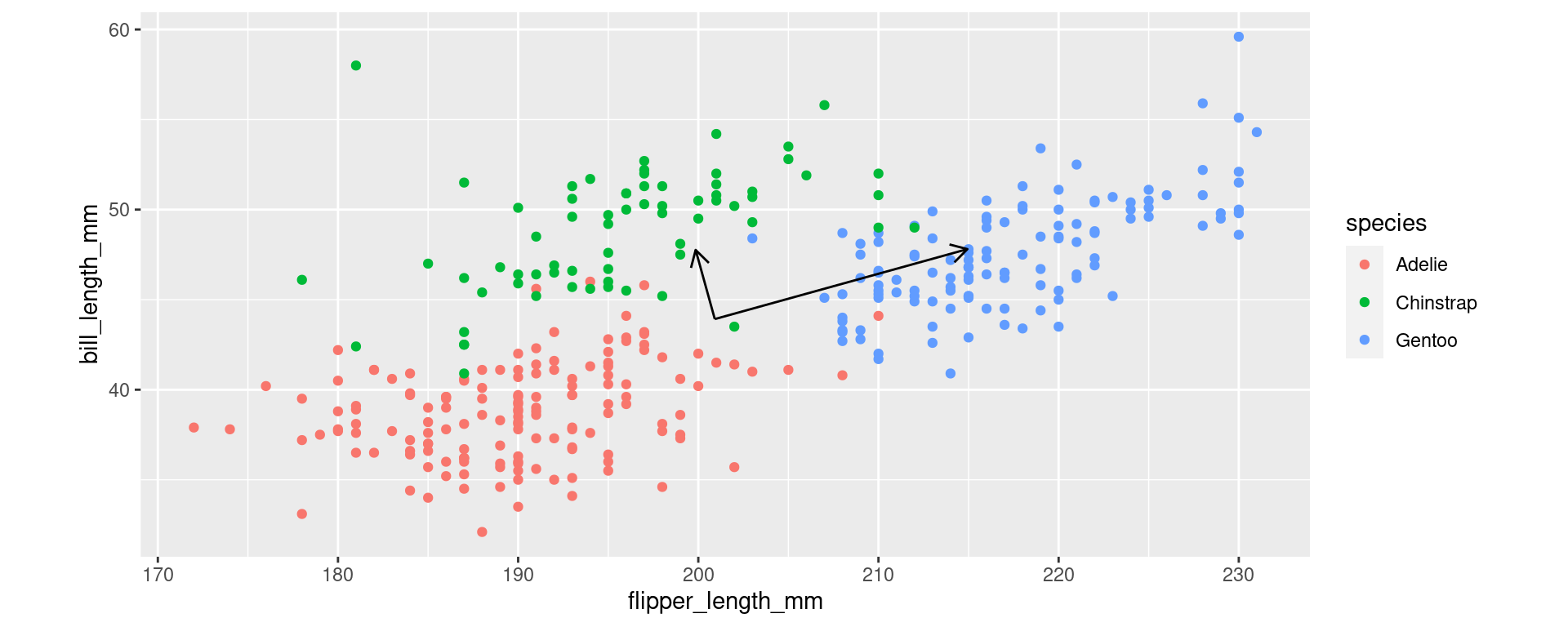
Two Variables

Example for the new axes.

The two arrows show the two eigenvectors of the covariance matrix of the two variables scaled by the square root of the corresponding eigenvalues, and shifted so their origins are at the means of both variables.

Computation in R

The basic function is base-R’s prcomp (there is an older princomp which is not advisable to use).

# prcomp can take a data frame with all numerical vectors as 1st argument
P <- peng |> select(flipper_length_mm, bill_length_mm) |> prcomp()

The base output

P

Standard deviations (1, .., p=2):
[1] 14.549388  3.981729

Rotation (n x k) = (2 x 2):
                        PC1        PC2
flipper_length_mm 0.9637169 -0.2669266
bill_length_mm    0.2669266  0.9637169

The summary output

summary(P)

Importance of components:
                           PC1     PC2
Standard deviation     14.5494 3.98173
Proportion of Variance  0.9303 0.06968
Cumulative Proportion   0.9303 1.00000

The prcomp object

Includes 4 different related entities.

The standard deviations related to each principal component.

P$sdev

[1] 14.549388  3.981729

The matrix of variable loadings. (It is also the matrix which rotates the original data vectors.)

P$rotation

                        PC1        PC2
flipper_length_mm 0.9637169 -0.2669266
bill_length_mm    0.2669266  0.9637169

The means for each original variable.

P$center

flipper_length_mm    bill_length_mm 
        200.91520          43.92193 

Note, there are also standard deviations of original variables in $scale when this is set to be used.

The centered (scaled, if set) and rotated data.

P$x

               PC1         PC2
  [1,] -20.4797199  0.66892267
  [2,] -15.5543649 -0.28022355
  [3,]  -6.6673719 -1.91158941
  [4,]  -9.5557414 -4.84711693
  [5,] -11.7528828 -1.54067330
  [6,] -20.5331052  0.47617930
  [7,]  -6.9609911 -2.97167796
  [8,] -10.2497505 -7.35278078
  [9,] -11.0321810  1.06136223
 [10,] -16.0081402 -1.91854222
 [11,] -21.7904413 -0.31698266
 [12,] -18.9821498  2.32942980
 [13,] -10.9760146 -2.48220170
 [14,]  -5.2977029 -8.20555532
 [15,] -17.2921689 -2.80807586
 [16,]  -7.0944544 -3.45353639
 [17,]  -4.1526997 -0.32526550
 [18,] -18.8431243 -4.66132637
 [19,]  -6.1096072  3.84852331
 [20,] -27.5727425  1.28457691
 [21,] -21.8171340 -0.41335434
 [22,] -13.6241501 -4.55038405
 [23,] -16.8650864 -1.26612888
 [24,] -21.5235147  0.64673421
 [25,] -15.7117398 -4.59476098
 [26,] -18.1518963  1.58064478
 [27,] -14.3237215  0.41656672
 [28,] -29.4734836  1.91480178
 [29,] -21.0697395  2.28505287
 [30,] -23.2640999  1.85518920
 [31,] -23.8780310 -0.36135959
 [32,] -13.6269312 -0.81407674
 [33,] -17.1081014  1.60283324
 [34,]  -7.7083856 -5.67008518
 [35,]  -5.9972743 -3.23860456
 [36,] -11.8863461 -2.02253174
 [37,] -20.6159643  3.92337154
 [38,] -20.8801098 -0.77665262
 [39,] -17.4017207  0.54274469
 [40,] -20.2100122 -2.10366777
 [41,]  -6.5339086 -1.42973098
 [42,] -16.4886080 -3.65323258
 [43,]  -4.6893340  1.48360808
 [44,] -17.1853983 -2.42258912
 [45,] -11.6728048 -1.25155824
 [46,] -18.9821498  2.32942980
 [47,] -22.8342362 -0.33917112
 [48,] -12.6337406 -4.72093895
 [49,]  -9.9883862  1.08355069
 [50,] -15.5276723 -0.18385187
 [51,] -13.4667753 -0.23584662
 [52,] -12.9006672 -5.68465582
 [53,]  -1.3950124 -1.60790371
 [54,] -15.9252810 -5.36573447
 [55,] -10.2286201  0.21620552
 [56,] -15.6878282 -0.76208199
 [57,]  -8.5147276 -1.08862116
 [58,] -21.1737290 -1.83674117
 [59,]  -8.3517906 -4.24669835
 [60,] -17.5324029 -3.67542104
 [61,]  -6.4004453 -0.94787255
 [62,] -17.0252423 -1.84435900
 [63,]  -9.3449812 -0.33983614
 [64,] -18.3092711 -2.73389264
 [65,]  -9.2115179  0.14202229
 [66,]  -7.9486195 -6.53743036
 [67,] -13.1998487  0.72787024
 [68,] -12.6604332 -4.81731064
 [69,]  -3.3758314 -1.26679390
 [70,] -13.3010571 -7.13023111
 [71,] -11.6461122 -1.15518656
 [72,]  -5.8905036 -2.85311781
 [73,]  -3.2718419  2.85500015
 [74,] -12.7672039 -5.20279739
 [75,]  -6.0000554  0.49770275
 [76,] -10.3620834 -0.26565292
 [77,] -18.0957298 -1.96291915
 [78,] -15.4715058 -3.72741580
 [79,]  -6.1869040 -0.17689906
 [80,] -13.9711547 -5.80321597
 [81,]  -5.0096459  0.32714784
 [82,] -15.3380425 -3.24555737
 [83,]  -9.9828239 -6.38906391
 [84,] -11.3230191 -3.73503363
 [85,]  -7.3641622 -0.68094595
 [86,] -12.5536626 -4.43182390
 [87,] -13.3572235 -3.58666718
 [88,] -12.9835263 -2.23746357
 [89,] -11.8596534 -1.92616005
 [90,]  -1.1492162 -8.21317314
 [91,]   3.1833380 -3.80988186
 [92,] -17.9861781 -5.31373971
 [93,] -15.5276723 -0.18385187
 [94,] -15.4715058 -3.72741580
 [95,]   5.9944106 -4.89977671
 [96,] -12.0731947 -2.69713354
 [97,]  -5.7036550 -2.17851601
 [98,] -24.9724301 -4.31259873
 [99,]  -8.7844354  1.68396928
[100,] -10.9732334 -6.21850901
[101,]   1.2292116 -3.37240036
[102,] -18.9259834 -1.21413413
[103,] -12.1532727 -2.98624860
[104,]  -9.2354294 -3.69065670
[105,] -17.4284133  0.44637301
[106,]  -3.2662796 -4.61761446
[107,] -12.0465021 -2.60076185
[108,] -20.7466465 -0.29479419
[109,]  -3.9658510  0.34933630
[110,]  -4.3634598 -4.83254629
[111,]  -9.1075284  4.26381634
[112,]  -8.7549616 -1.95596634
[113,]  -4.2327776 -0.61438056
[114,] -10.7090880 -1.51848484
[115,]  -5.0630312  0.13440447
[116,] -13.8671651 -1.68142192
[117,]  -3.6132842 -5.87044638
[118,] -13.6775354 -4.74312742
[119,] -12.2361318  0.46094364
[120,] -15.4715058 -3.72741580
[121,]  -4.4702304 -5.21803304
[122,] -25.0046850  3.06364419
[123,]   0.3722654 -2.71998702
[124,] -16.7021493 -4.42420607
[125,]  -2.7324265 -2.69018073
[126,] -10.9226292 -2.28945833
[127,]  -6.3470600 -0.75512918
[128,] -10.8692439 -2.09671496
[129,]   8.8027021 -2.25336424
[130,] -11.9664241 -2.31164679
[131,]  -3.9925437  0.25296462
[132,]  -9.5290487 -4.75074525
[133,]  -3.5598989 -5.67770301
[134,] -14.9643453 -1.89635376
[135,] -11.2724149  0.19401705
[136,] -11.7767943 -5.37335229
[137,]  -1.8754802 -3.34259407
[138,] -17.1853983 -2.42258912
[139,]  -8.7549616 -1.95596634
[140,]  -8.6214983 -1.47410791
[141,] -14.2970288  0.51293840
[142,] -15.6021880 -7.94558153
[143,] -11.3791856 -0.19146969
[144,] -10.3593023 -4.00196022
[145,] -16.6515451 -0.49515539
[146,] -11.7795755 -1.63704499
[147,] -18.2558858 -2.54114927
[148,]  -7.8151562 -6.05557193
[149,]  -9.2621221 -3.78702838
[150,] -15.5248912 -3.92015917
[151,]  -0.5647588 -2.35668874
[152,]  10.3002722 -0.59285711
[153,]  29.6519063 -1.90596663
[154,]  10.0305645  2.17973333
[155,]  18.0873039  1.29715250
[156,]  14.5555295 -0.21498819
[157,]   9.4433259  0.05955623
[158,]  10.1134236 -1.26745892
[159,]  18.1701630 -2.15003975
[160,]   7.6254440 -2.75741114
[161,]  14.3419882 -0.98596168
[162,]  11.8034045 -6.40496458
[163,]  15.8929436  0.86728882
[164,]  13.0312668 -1.97186701
[165,]  12.8416371  1.08983849
[166,]   9.2564773 -0.61504558
[167,]  16.9367385  0.88947729
[168,]   8.2421563 -4.27716966
[169,]  20.7649133 -0.27460078
[170,]   8.3995311  0.03736776
[171,]  21.5951668 -1.02338580
[172,]  18.1406893  1.48989587
[173,]  13.8882130 -2.62428035
[174,]  12.3344765 -0.74122355
[175,]  14.2085249 -1.46782012
[176,]  13.3009745 -4.74445745
[177,]  14.1551396 -1.66056349
[178,]  14.6917739 -3.46943706
[179,]  14.6089148 -0.02224482
[180,]   9.8971012  1.69787490
[181,]  20.0147377  0.76329931
[182,]  21.2214696 -2.37258941
[183,]   7.4919807 -3.23926957
[184,]   6.1784781 -0.48886760
[185,]  32.2144016  7.34571526
[186,]  19.7745037 -0.10404587
[187,]  19.5876551 -0.77864767
[188,]  11.2934628 -4.49971932
[189,]  17.5562319 -4.36658853
[190,]   6.8485757 -1.81588274
[191,]   8.1031307  2.71358652
[192,]   6.5015712 -3.06871466
[193,]  24.7265513 -0.95682041
[194,]   9.1230140 -1.09690401
[195,]  16.0530996  1.44551894
[196,]  22.0756347  0.71130455
[197,]  15.4152569 -4.60370884
[198,]   9.1763994 -0.90416063
[199,]  24.9667853 -0.08947523
[200,]  11.9073940 -2.28317054
[201,]  13.9149057 -2.52790867
[202,]   9.4700186  0.15592792
[203,]  19.6143478 -0.68227599
[204,]   9.0696287 -1.28964738
[205,]  24.8600146 -0.47496198
[206,]  16.1893440 -1.80892993
[207,]  18.6801047 -4.05528501
[208,]   6.7951904 -2.00862611
[209,]  18.8135680 -3.57342658
[210,]   6.6350345 -2.58685623
[211,]  23.9763758  0.08107968
[212,]   7.1955803 -0.56305082
[213,]  19.9641335 -3.16575137
[214,]  13.0846521 -1.77912364
[215,]  31.7634075  1.97108929
[216,]  17.9299291 -3.01738492
[217,]  29.5985210 -2.09871001
[218,]  13.2181154 -1.29726521
[219,]  28.5547261 -2.12089847
[220,]  18.2797148 -5.50086030
[221,]  23.0927369  0.63712133
[222,]  15.5459390 -0.38554310
[223,]  20.0175188 -2.97300799
[224,]  20.4979867 -1.23831764
[225,]  16.1893440 -1.80892993
[226,]  15.1989345 -1.63837502
[227,]  29.2782091 -3.25517024
[228,]   8.7465357  1.29019969
[229,]  20.3083569  1.82338786
[230,]  13.9149057 -2.52790867
[231,]  21.6246406 -4.66332142
[232,]  12.0647688  2.03136689
[233,]  21.6457710  2.90566487
[234,]  11.6109936  0.39304822
[235,]  23.8696051 -0.30440707
[236,]  10.9436771 -2.01624394
[237,]  27.9380138 -0.60113995
[238,]  16.3255884 -5.06337880
[239,]  18.4343085  2.54998442
[240,]  11.6376863  0.48941990
[241,]  30.2124521  0.11783878
[242,]  17.4199874 -1.11213966
[243,]  28.3117111  0.74806366
[244,]  11.1038331 -1.43801382
[245,]  23.7361418 -0.78626550
[246,]  12.7643402 -2.93558388
[247,]  26.0105801 -0.06728677
[248,]  15.9997143  1.25277557
[249,]  21.1146989 -2.75807616
[250,]   3.2044684  3.75910443
[251,]  25.1269412  0.48875489
[252,]  18.6506309 -0.41534939
[253,]  29.2993395  4.31381605
[254,]  14.4487589 -0.60047494
[255,]  27.4842386 -2.23945862
[256,]  15.4391684 -0.77102985
[257,]  14.3419882 -0.98596168
[258,]   8.1620783 -4.56628472
[259,]  19.9585712  4.30686324
[260,]   6.6617271 -2.49048455
[261,]   8.9066916  1.86842981
[262,]  16.2933335  2.31286412
[263,]  28.6348041 -1.83178341
[264,]  11.5336968 -3.63237414
[265,]  30.0522962 -0.46039134
[266,]  16.1092660 -2.09804499
[267,]  31.0132319  3.00898937
[268,]  15.6554908 -3.73636366
[269,]  21.6218595 -0.92701412
[270,]  13.4850420 -0.33354834
[271,]  14.3419882 -0.98596168
[272,]  22.0489420  0.61493287
[273,]  11.0237551 -1.72712888
[274,]  13.2420270  2.53541378
[275,]  -7.9035776  4.86423493
[276,]  -3.1144671  7.16953757
[277,]  -5.6586131  9.22314928
[278,] -12.0520643  4.87185275
[279,]  -1.4300484  9.50464651
[280,]  -2.4682810  2.00984344
[281,] -21.5023843  8.21572050
[282,]  -1.8037456  8.15544290
[283,]  -5.1458903  3.58159671
[284,]  -0.8400288  7.88851631
[285,]  -6.9131681  4.69368002
[286,]  -4.5881256  9.34170943
[287,] -14.5161323  7.21457952
[288,]   2.2379704  7.76233833
[289,]  -9.9911673  4.81985800
[290,]   1.8375806  6.31676303
[291,]  -2.0706722  7.19172604
[292,] -15.4348073 18.88317139
[293,]  -9.8577040  5.30171643
[294,]  -4.2917252  6.66549067
[295,] -19.5988621  3.84918832
[296,]  -8.3334413  7.05859525
[297,] -13.6030197  3.01860225
[298,]  -5.8454617  8.54854747
[299,]  -4.9590417  4.25619852
[300,]  -1.6168970  8.83004470
[301,]   0.8738637  6.58368963
[302,]   0.6069371  5.61997276
[303,]  -8.8939871  5.03478983
[304,]   6.3063792  7.46560544
[305,] -14.2169508  0.80205346
[306,]   2.8252089  9.88251543
[307,] -13.7898683  2.34400044
[308,]   3.8984776  6.26476828
[309,]  -4.1582619  7.14734911
[310,]  -0.8906330  3.95946563
[311,]  -4.7188078  5.12354369
[312,]  10.9114222  5.35999898
[313,]  -7.7968070  5.24972167
[314,]   6.4932278  8.14020725
[315,]  10.1106424  2.46884839
[316,] -12.8022399  5.90975284
[317,]  -2.8742331  8.03688275
[318,]  -4.3156367  2.83281168
[319,]  -2.8742331  8.03688275
[320,]   1.9176585  6.60587809
[321,]  -8.8700756  8.86746882
[322,]  12.0380762  1.93499520
[323,] -11.3875289 11.01745222
[324,]  -1.2404187  6.44294101
[325,]  -0.7304770  4.53769575
[326,]   2.0778145  7.18410821
[327,]  -7.1534020  3.82633484
[328,]   3.8183996  5.97565322
[329,] -13.7898683  2.34400044
[330,]  -1.5635117  9.02278808
[331,]  -9.2142990  3.87832960
[332,]   3.4447024  4.62644961
[333,]   2.7212194  5.76072138
[334,]  -6.2163778  3.46303656
[335,]   7.0298621  6.33133367
[336,] -10.7146502  5.95412977
[337,]  -5.2259683  3.29248165
[338,]   9.0345927  9.82290284
[339,]   0.9328113 -0.69618161
[340,]  -6.1123883  7.58483061
[341,]  10.5911103  4.20353874
[342,]  -1.1336480  6.82842776

PCA as Exploratory Data Analysis

Suppose we do a PCA with all 342 penguins (rows) and all 4 numeric variables.

• How long will the vector of standard deviations be? 4
  
• What dimensions will the rotation matrix have? 4 x 4
  
• What dimensions will the rotated data frame have? 342 x 4

When we do a PCA for exploration there are 3 things to look at:

1. The data in PC coordinates - the centered (scaled, if set) and rotated data.
   
2. The rotation matrix - the variable loadings.
3. The variance explained by each PC - based on the standard deviations.

All variables

Now, with scale = TRUE (recommended). Data will be centered and scaled (a.k.a. standardized) first.

peng_PCA <- peng |> select(-species) |> 
 prcomp(scale = TRUE)
peng_PCA

Standard deviations (1, .., p=4):
[1] 1.6594442 0.8789293 0.6043475 0.3293816

Rotation (n x k) = (4 x 4):
                         PC1          PC2        PC3        PC4
bill_length_mm     0.4552503 -0.597031143 -0.6443012  0.1455231
bill_depth_mm     -0.4003347 -0.797766572  0.4184272 -0.1679860
flipper_length_mm  0.5760133 -0.002282201  0.2320840 -0.7837987
body_mass_g        0.5483502 -0.084362920  0.5966001  0.5798821

Explore data in PC coordinates

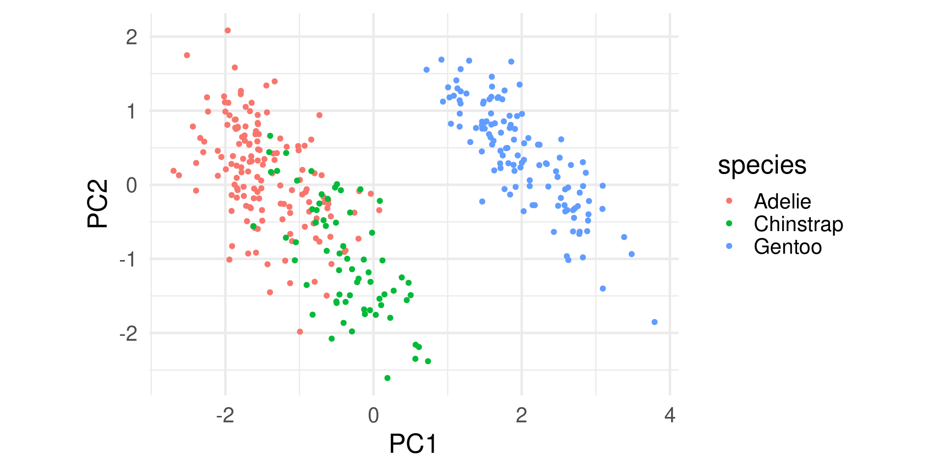
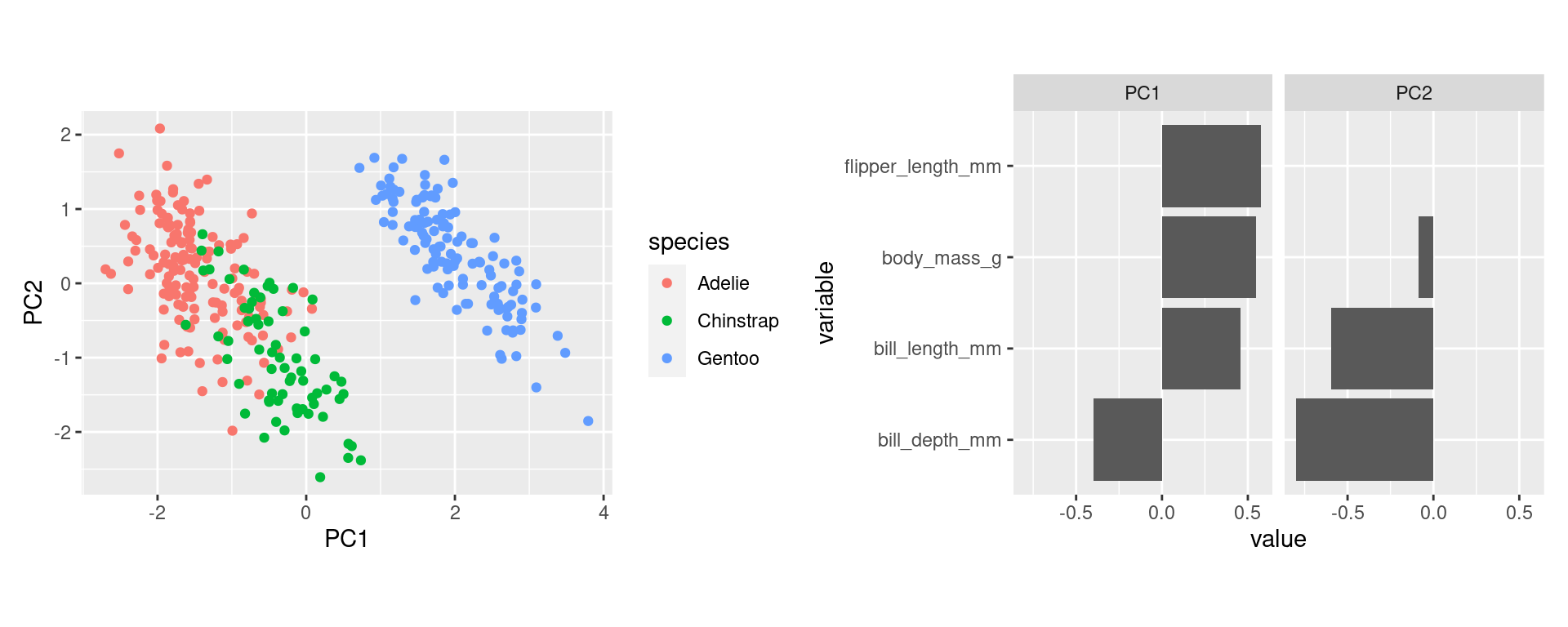
• Start plotting PC1 against PC2. By default these are the most important ones. Drill deeper later.
• Append the original data. Here used to color by species.

plotdata <- peng_PCA$x |> as_tibble() |> bind_cols(peng)
plotdata |> ggplot(aes(PC1, PC2, color = species)) +
 geom_point() +
 coord_fixed() + theme_minimal(base_size = 20)

Variable loadings

• The columns of the rotation matrix shows how the original variables load on the principle components.
• We can try to interpret these loadings and give descriptive names to principal components.
• tidy extracts the rotation matrix in long format with a PC, a column (for the original variable name), and a value variable.

peng_PCA$rotation |> as_tibble(rownames = "variable") |> 
 pivot_longer(starts_with("PC"), names_to = "PC", values_to = "value") |> 
 ggplot(aes(value, variable)) + geom_col() + geom_vline(xintercept = 0, color = "blue") +
 facet_wrap(~PC, nrow = 1) + theme_minimal(base_size = 20)

Variance explained

• Principle components are by default sorted by importance.
• The squares of the standard deviation for each component gives its variances and variances have to sum up to the sum of the variances of the original variables.
  • When original variables were standardized their original variances are all each one. Consequently, the variances of the principal components sum up to the number of original variables.
• A typical plot to visualize the importance of the components is to plot the percentage of the variance explained by each component.

tibble(PC = 1:4, sdev = peng_PCA$sdev) |> 
 mutate(percent = sdev^2/sum(sdev^2) * 100) |>
 ggplot(aes(PC, percent)) + geom_col() + theme_grey(base_size = 20)

Interpretations (1)

• The first component explains almost 70% of the variance. So most emphasize should be on this.
• The first two explain about 88% of the total variance.

Interpretations (2)

1. To score high on PC1 a penguin needs to be generally large but with low bill depth.
2. Penguins scoring high on PC2 are penguins with generally small bills.

Interpretations (3)

Apply PCA

• Besides standardization, PCA may benefit by preprocessing steps of data transformation with variables with skew distributions (log, square-root, or Box-Cox transformation). This may result in less outliers.
• PCA is a often a useful step of exploratory data analysis when you have a large number of numerical variables to show the empirical dimensionality of the data and its structure
• Limitation: PCA is only sensitive for linear relation ships (no U-shaped) or the like
• The principal components can be used as predictors in a model instead of the raw variables.

Properties of PCA

• The principal components (the columns of the rotation matrix) are maximally uncorrelated (actually they are even orthogonal).
• This also holds for the columns of the rotated data.
• The total variances of all prinicipal components sum up to the number of variables (when variables are standardized)
• The PCA is unique. All principle components together are a complete representation of the data. (Unlike other technique of dimensionality reduction which may rely on starting values, random factors, or tuning parameters)

Relations of PCA

• A technique similar in spirit is factor analysis (e.g. factanal). It is more theory based as it requires to specify to the theoriezed number of factors up front.
• PCA is an example of the importance of linear algebra (“matrixology”) in data science techniques.
  • PCA is based on the eigenvalue decomposition of the covariance matrix (or correlation matrix in the standardized case) of the data.