W#04: Math refresh, Function Programming, Descriptive Statistics

Jan Lorenz

Math: Sets and vectors

Definition: Sets and vectors

A set is mathematical model for the collection of different things.

Examples

• \(\{3, \text{Hi}, 😀, 🖖 \}\)
• \(\{1,3,5\}\)
• The natural numbers \(\mathbb{N} = \{1, 2, 3, \dots\}\) (infinite!)
• \(\{\mathtt{"EWR"}, \mathtt{"LGA"}, \mathtt{"JFK"}\}\)
  these are origin airports in flights

Math: Sets and vectors

A vector is an ordered collection of things (elements) of the same type.

In a set each thing can only be once and the order does not matter!

\(\{1,3,5\} = \{3,5,1\} = \{1,1,1,3,5,5\}\)

For vectors:

\([1\ 3\ 5] \neq [3\ 5\ 1]\) because we compare component-wise, so we cannot even compare with those with the vector \([1\ 1\ 1\ 3\ 5\ 5]\)

Math: Set operations

Sets \(A = \{🐺, 🦊, 🐶\}\) and \(B = \{🐶, 🐷, 🐹\}\), \(C = \{🐶, 🐷\}\):

• Set union \(A \cup B\) = {🐺, 🦊, 🐶, 🐷, 🐹}
  \(x \in A \cup B\) when \(x \in A\) | (or) \(x\in B\)
• Set intersection \(A \cap B\) = {🐶}
  \(x \in A \cap B\) when \(x \in A\) & (and) \(x\in B\)
• Set difference \(A \setminus B = \{🐺, 🦊\}\), \(B \setminus A\) = {🐷, 🐹}
• Subset: \(C \subset B\) but \(C \not\subset A\)

See the analogy of set operations and logical operations.

Set operations in R

unique shows the set of elements in a vector

unique(flights$origin)

[1] "EWR" "LGA" "JFK"

setequal tests for set equality

setequal(c("EWR","LGA","JFK"), c("EWR","EWR","LGA","JFK"))

[1] TRUE

union, intersect, setdiff treat vectors as sets and operate as expected

union(1:5,3:7)

[1] 1 2 3 4 5 6 7

intersect(1:5,3:7)

[1] 3 4 5

setdiff(1:5,3:7)

[1] 1 2

Sets: Take-away

• Set operations are not a daily business in data science
• However, they are useful for data exploration!
• Knowing set operations is key to understand probability:
  • A sample space is the set of all atomic events.
  • An event is a subset of the sample
  • A probability function assigns probabilities to all events.

Math: Functions

Functions mathematically

Consider two sets: The domain \(X\) and the codomain \(Y\).

A function \(f\) assigns each element of \(X\) to exactly one element of \(Y\).

We write \(f : X \to Y\)
“\(f\) maps from \(X\) to \(Y\)”

and \(x \mapsto f(x)\)
“\(x\) maps to \(f(x)\)”

The yellow set is called the image of \(f\).

Picture from wikipedia.

Conventions in mathematical text

• Sets are denoted with capital letters.
• Their elements with (corresponding) small letters.
• Functions are often called \(f\), \(g\), or \(h\).
• Other terminology can be used!

Important in math

• When you read math:
  Keep track of what objects are! What are functions, what are sets, what are numbers, …¹
• When you write math: Define what objects are.

1. Watch: How to read math https://www.youtube.com/watch?v=Kp2bYWRQylk

Is this a mathematical function?

\(\ \mapsto\ \)

Input from \(X = \{\text{A picture where a face can be recognized}\}\).

Function: Upload input at https://funny.pho.to/lion/ and download output.

Output from \(Y = \{\text{Set of pictures with a specific format.}\}\)

Yes, it is a function. Important: Output is the same for the same input!

Is this a mathematical function?

Input a text snippet. Function: Enter text at https://www.craiyon.com. Output a picture.

Other examples:

• “Nuclear explosion broccoli”
• “The Eye of Sauron reading a newspaper”
• “The legendary attack of Hamster Godzilla wearing a tiny Sombrero”

No, it is not a function. It has nine outcomes and these change when run again.

Graphs of functions

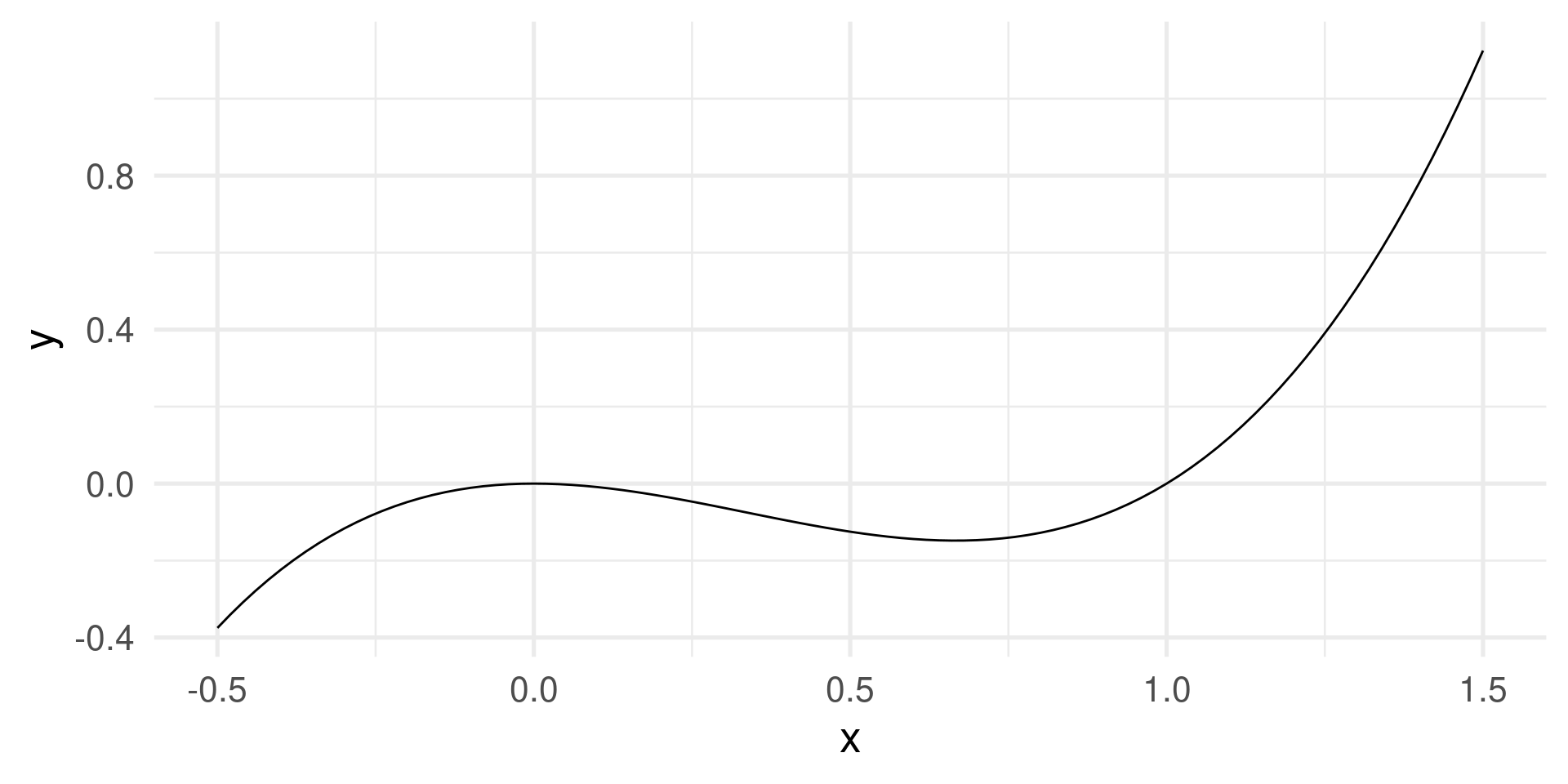
• A function is characterized by the set all possible pairs \((x,f(x))\).
• This is called its graph.
• When domain and codomain are real numbers then the graph can be shown in a Cartesian coordinate system. Example \(f(x) = x^3 - x^2\)

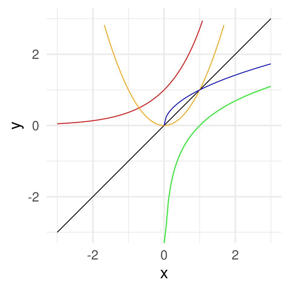
Some functions \(f: \mathbb{R} \to \mathbb{R}\)

\(f(x) = x\) identity function
\(f(x) = x^2\) square function
\(f(x) = \sqrt{x}\) square root function
\(f(x) = e^x\) exponential function
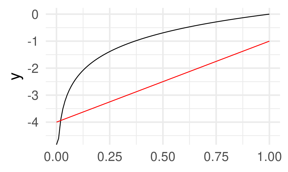
\(f(x) = \log(x)\) natural logarithm

• Square and square root function are inverse of each other. Exponential and natural logarithm, too.

\(\sqrt[2]{x}^2 = \sqrt[2]{x^2} = x\), \(\log(e^x) = e^{\log(x)} = x\)

• Identity function graph as mirror axis.

\(e\) is Euler’s number \(2.71828\dots\). The natural logarithm is also often called \(\ln\). The square root function is \(\mathbb{R}_{\geq 0} \to \mathbb{R}\), the logarithm \(\mathbb{R}_{>0} \to \mathbb{R}\).

Shifts and scales

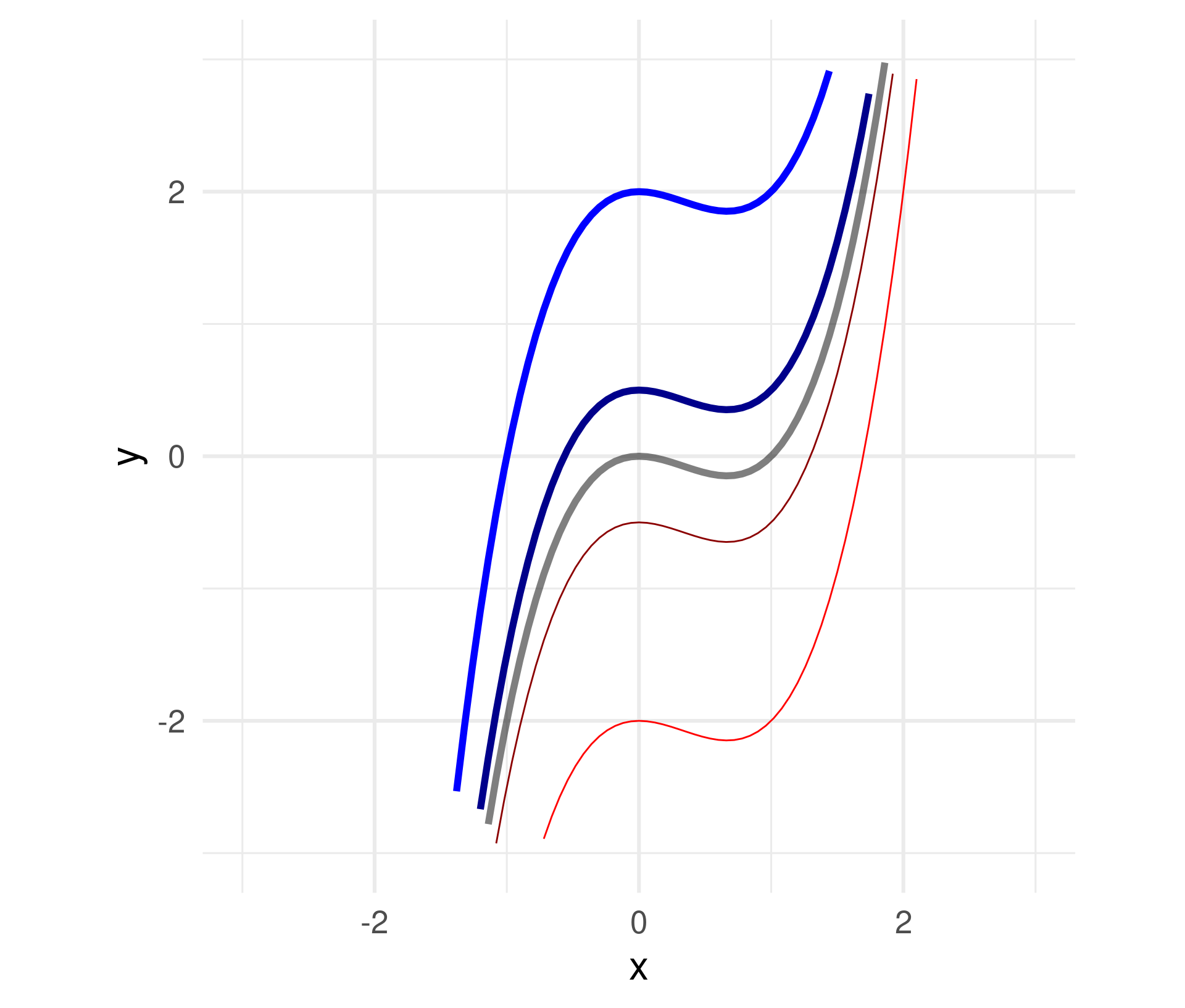
How can we shift, stretch, or shrink a graph vertically and horizontally?

• \(y\)-shift
• \(x\)-shift
• \(y\)-scale
• \(x\)-scale

Add a constant to the function.

\(f(x) = x^3 - x^2 \leadsto\)

\(\quad f(x) = x^3 - x^2 + a\)

For \(a =\) -2, -0.5, 0.5, 2

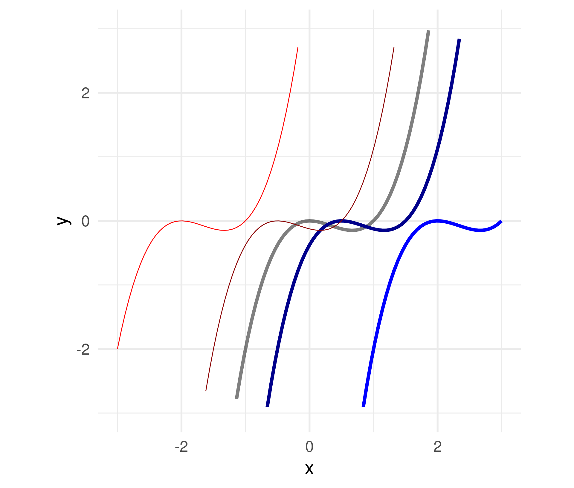
Subtract a constant from all \(x\) within the function definition.

\(f(x) = x^3 - x^2 \leadsto\)

\(\quad f(x) = (x - a)^3 - (x - a)^2\)

For \(a =\) -2, -0.5, 0.5, 2

Attention:
Shifting \(a\) units to the right needs subtracting \(a\)!
You can think of the coordinate system being shifted in direction \(a\) while the graph stays.

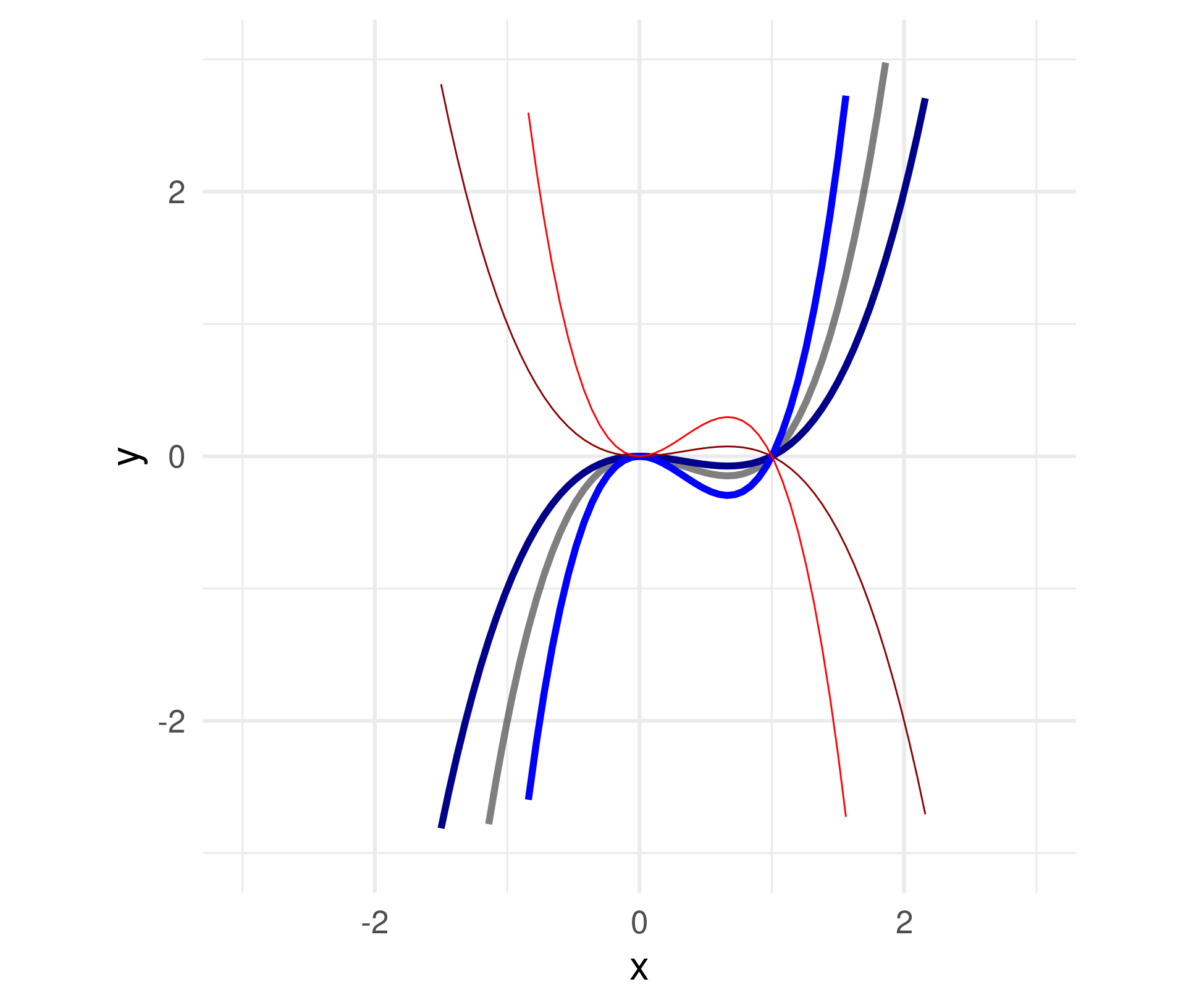
Multiply a constant to all \(x\) within the function definition.

\(f(x) = x^3 - x^2 \leadsto\)

\(\quad f(x) = a(x^3 - x^2)\)

For \(a =\) -2, -0.5, 0.5, 2

Negative numbers flip the graph around the \(x\)-axis.

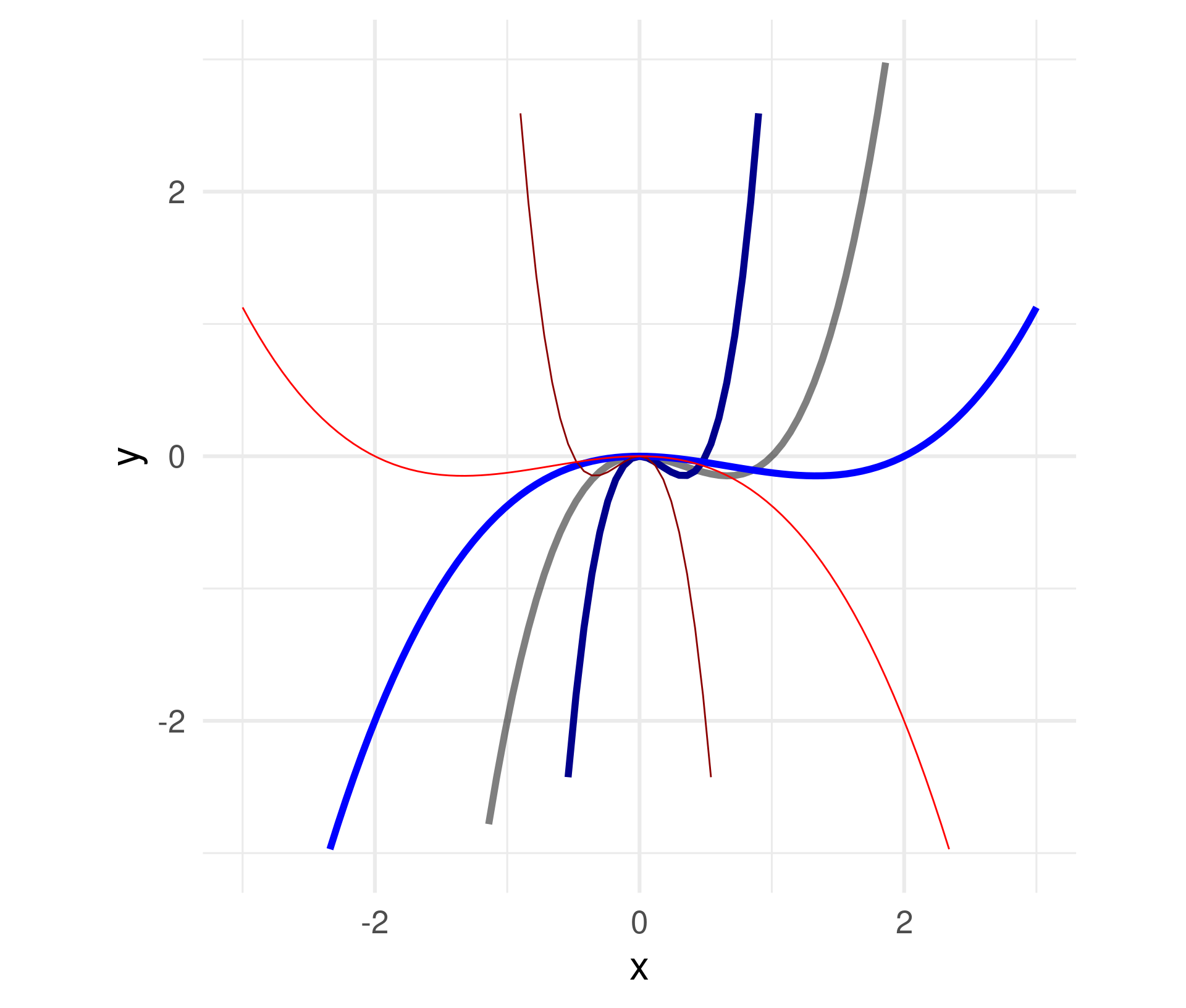
Divide all \(x\) within the function definition by a constant.

\(f(x) = x^3 - x^2 \leadsto\)

\(\quad f(x) = (x/a)^3 - (x/a)^2\)

For \(a =\) -2, -0.5, 0.5, 2

Negative numbers flip the graph around the \(y\)-axis.

Attention: Stretching needs a division by \(a\)!
You can think of the coordinate system being stretched multiplicatively by \(a\) while the graph stays.

Math: Polynomials and exponentials

A polynomial is a function which is composed of (many) addends of the form \(ax^n\) for different values of \(a\) and \(n\).

In an exponential the \(x\) appears in the exponent.

\(f(x) = x^3\) vs. \(f(x) = e^x\)

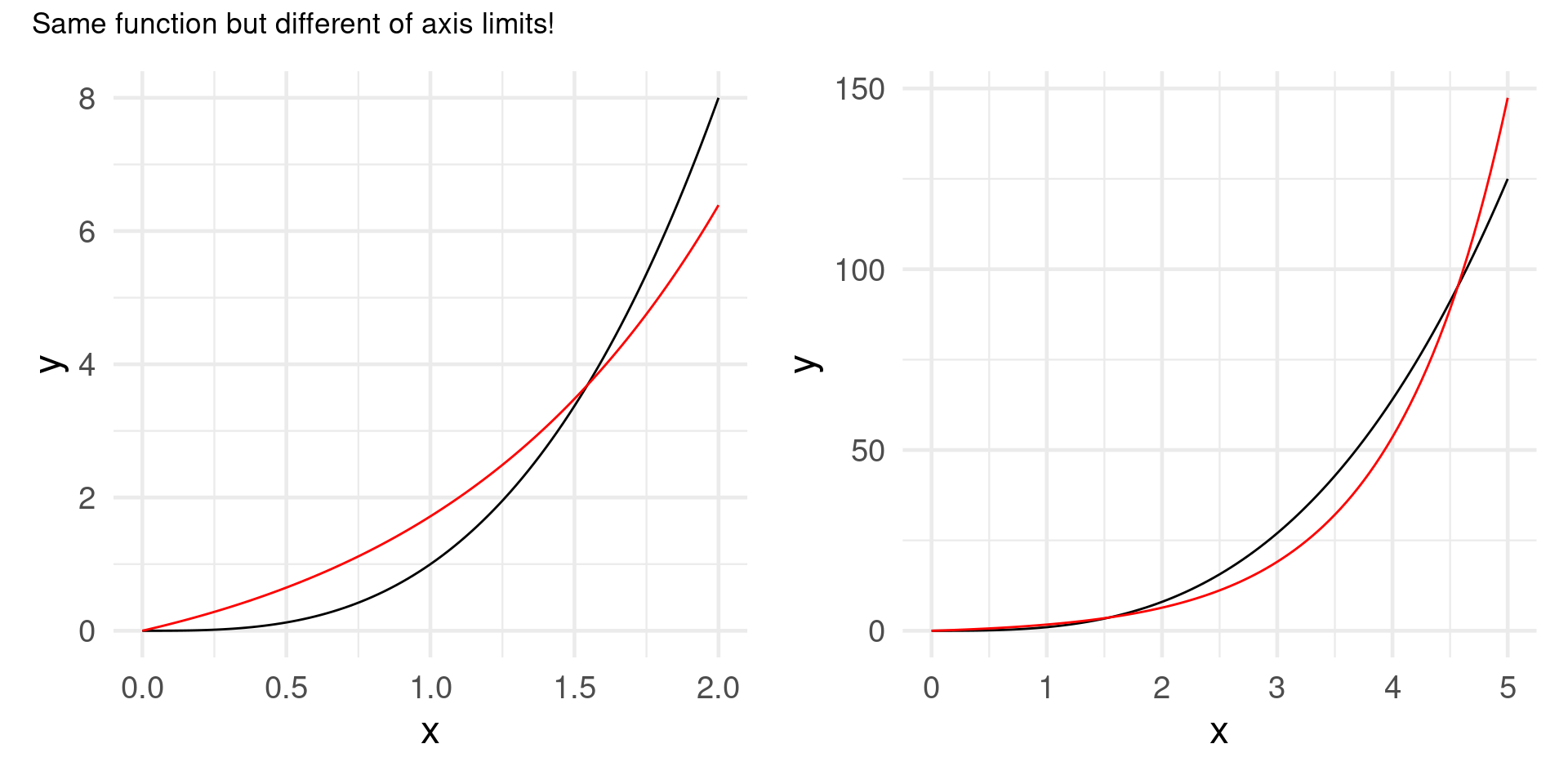
For \(x\to\infty\), any exponential will finally “overtake” any polynomial.

Math: Exponentiations and logarithms

Rules for exponentiation

\(x^0\)

\(0^x\)

\(0^0\)

\((x\cdot y)^a\)

\(x^{-a}\), \(x^{-1}\)

\(x^\frac{a}{b}\), \(x^\frac{1}{2}\)

\((x^a)^b\)

\(x^0 = 1\)

\(0^x = 0\) for \(x\neq 0\)

\(0^0 = 1\) (discontinuity in \(0^x\))

\((x\cdot y)^a = x^a\cdot x^b\)

\(x^{-a} = \frac{1}{x^a}\), \(x^{-1} = \frac{1}{x}\)

\(x^\frac{a}{b} = \sqrt[b]{x^a} = (\sqrt[b]{x})^a,\ x^\frac{1}{2} = \sqrt{x}\)

\((x^a)^b = x^{a\cdot b} = (x^b)^a \neq x^{a^b} = x^{(a^b)}\)
Example: \((4^3)^2 = 64^2 = 4096 \qquad 4^{3^2} = 4^9 = 262144\)

More rules for exponentiation

\(x^a\cdot x^b\)

\(x^a\cdot x^b = x^{a+b}\) Multiplication of powers (with same base \(x\)) becomes addition of exponents.

\((x+y)^a\)

No “simple” form! For \(a\) integer use binomial expansion. \((x+y)^2 = x^2 + 2xy + y^2\)
\((x+y)^3 = x^3 + 3x^2y + 3xy^2 + y^3\)
\((x+y)^n = \sum_{k=0}^n {n \choose k} x^{n-k}y^k\)

Pascal’s triangle

From wikipedia

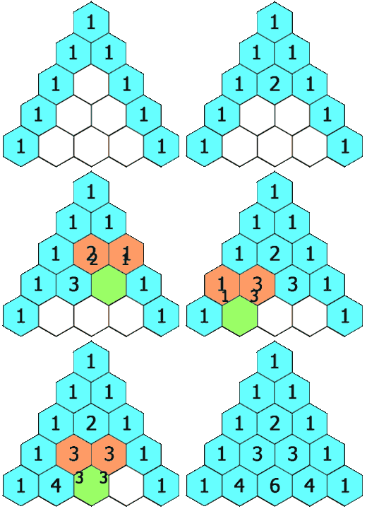
We meet it again in Probability:
A row represents a binomial distribution
Which tends to mimics the normal distribution more and more
and is related to the central limit theorem

Logarithms

Definition: A logarithm of \(a\) for some base \(b\) is the value of the exponent which brings \(b\) to \(a\): \(\log_b(a) = x\) means that \(b^x =a\)

Most common:

• \(\log_{10}\) useful for plotting data in logarithmic scales because the numbers can be interpreted easiest (number of decimals of the original values)
• \(\log_{e}\) natural logarithm (also \(\log\) or \(\ln\)) useful in calculus and statistics because of nice mathematical properties

\(\log_{10}(100) =\)

\(2\)

\(\log_{10}(1) =\)

\(0\)

\(\log_{10}(6590) =\)

\(3.818885\)

\(\log_{10}(0.02) =\)

\(-1.69897\)

Rules for logarithms

Usually only one base is used in the same context, because changing base is easy:

\(\log_c(x) = \frac{\log_b(x)}{\log_b(c)} = \frac{\log(x)}{\log(c)}\)

\(\log(x\cdot y)\)

\(= \log(x) + \log(y)\) Multiplication \(\to\) addition.

\(\log(x^y)\)

\(= y\cdot\log(x)\)

\(\log(x+y)\)

complicated!

Also changing bases for powers is easy: \(x^y = (e^{\log(x)})^y = e^{y\cdot\log(x)}\)

Functions in Programming

Input \(\to\) output

• Metaphorically, a function is a machine or a blackbox that for each input yields an output.
• The inputs of a function are also called arguments.

Difference to math terminolgy:
The output need not be the same for the same input.

Picture from wikipedia.

Function as objects in R

function is a class of an object in R

class(c)

[1] "function"

class(ggplot2::ggplot)

[1] "function"

Calling the function without brackets writes its code or some information.

sd # This function is written in R, and we see its code

function (x, na.rm = FALSE) 
sqrt(var(if (is.vector(x) || is.factor(x)) x else as.double(x), 
    na.rm = na.rm))
<bytecode: 0x55b0c7b79b98>
<environment: namespace:stats>

c # This function is not written in R but is a R primitive

function (...)  .Primitive("c")

ggplot2::ggplot # This function is not written solely in R

function (data = NULL, mapping = aes(), ..., environment = parent.frame()) 
{
    UseMethod("ggplot")
}
<bytecode: 0x55b0c6cd1ae8>
<environment: namespace:ggplot2>

Define your own functions! (in R)

add_one <- function(x) {
  x + 1 
}
# Test it
add_one(10)

[1] 11

The skeleton for a function definition is

function_name <- function(input){
  # do something with the input(s)
  # return something as output
}

• function_name should be a short but evocative verb.
• The input can be empty or one or more name or name=expression terms as arguments.
• The last evaluated expression is returned as output.
• When the body or the function is only one line {} can be omitted. For example
  add_one <- function(x) x + 1

Flexibility of inputs and outputs

• Arguments can be specified by name=expression or just expression (then they are taken as the next argument)
• Default values for arguments can be provided. Useful when an argument is a parameter.

mymult <- function(x = 2, y = 3) x * (y - 1)
mymult(3,4)

[1] 9

mymult()

[1] 4

mymult(y = 3, x = 6)

[1] 12

mymult(5)

[1] 10

mymult(y = 2)

[1] 2

For complex output use a list

mymult <- function(x = 2, y = 3) 
  list(out1 = x * (y - 1), out2 = x * (y - 2))
mymult()

$out1
[1] 4

$out2
[1] 2

Vectorized functions

Mathematical functions in programming are often “vectorized”:

• Operations on a single value are applied to each component of the vector.
• Operations on two values are applied “component-wise” (for vectors of the same length)

log10(c(1,10,100,1000,10000))

[1] 0 1 2 3 4

c(1,1,2) + c(3,1,0)

[1] 4 2 2

(0:5)^2

[1]  0  1  4  9 16 25

Recall: Vector creation functions

1:10

 [1]  1  2  3  4  5  6  7  8  9 10

seq(from=-0.5, to=1.5, by=0.1)

 [1] -0.5 -0.4 -0.3 -0.2 -0.1  0.0  0.1  0.2  0.3  0.4  0.5  0.6  0.7  0.8  0.9
[16]  1.0  1.1  1.2  1.3  1.4  1.5

seq(from=0, to=1, length.out=10)

 [1] 0.0000000 0.1111111 0.2222222 0.3333333 0.4444444 0.5555556 0.6666667
 [8] 0.7777778 0.8888889 1.0000000

rep(1:3, times=3)

[1] 1 2 3 1 2 3 1 2 3

rep(1:3, each=3)

[1] 1 1 1 2 2 2 3 3 3

Plotting and transformation

Vector creation and vectorized functions are key for plotting and transformation.

func <- function(x) x^3 - x^2    # Create a vectorized function
data <- tibble(x = seq(-0.5,1.5,by =0.01)) |>    # Vector creation
    mutate(y = func(x))        # Vectorized transformation using the function
data |> ggplot(aes(x,y)) + geom_line() + theme_minimal(base_size = 20)

Conveniently ggploting functions

ggplot() +
 geom_function(fun = log) +
 geom_function(fun = function(x) 3*x - 4, color = "red") +
 theme_minimal(base_size = 20)

Line 3 shows another important concept: anonymous functions. The function function(x) 3*x - 4 is defined on the fly without a name.

Conditional statements

• if executes a code block if a condition is TRUE
• else executes a code block if the condition is FALSE

Skeleton

if (condition) {
  # code block
} else {
  # code block
}

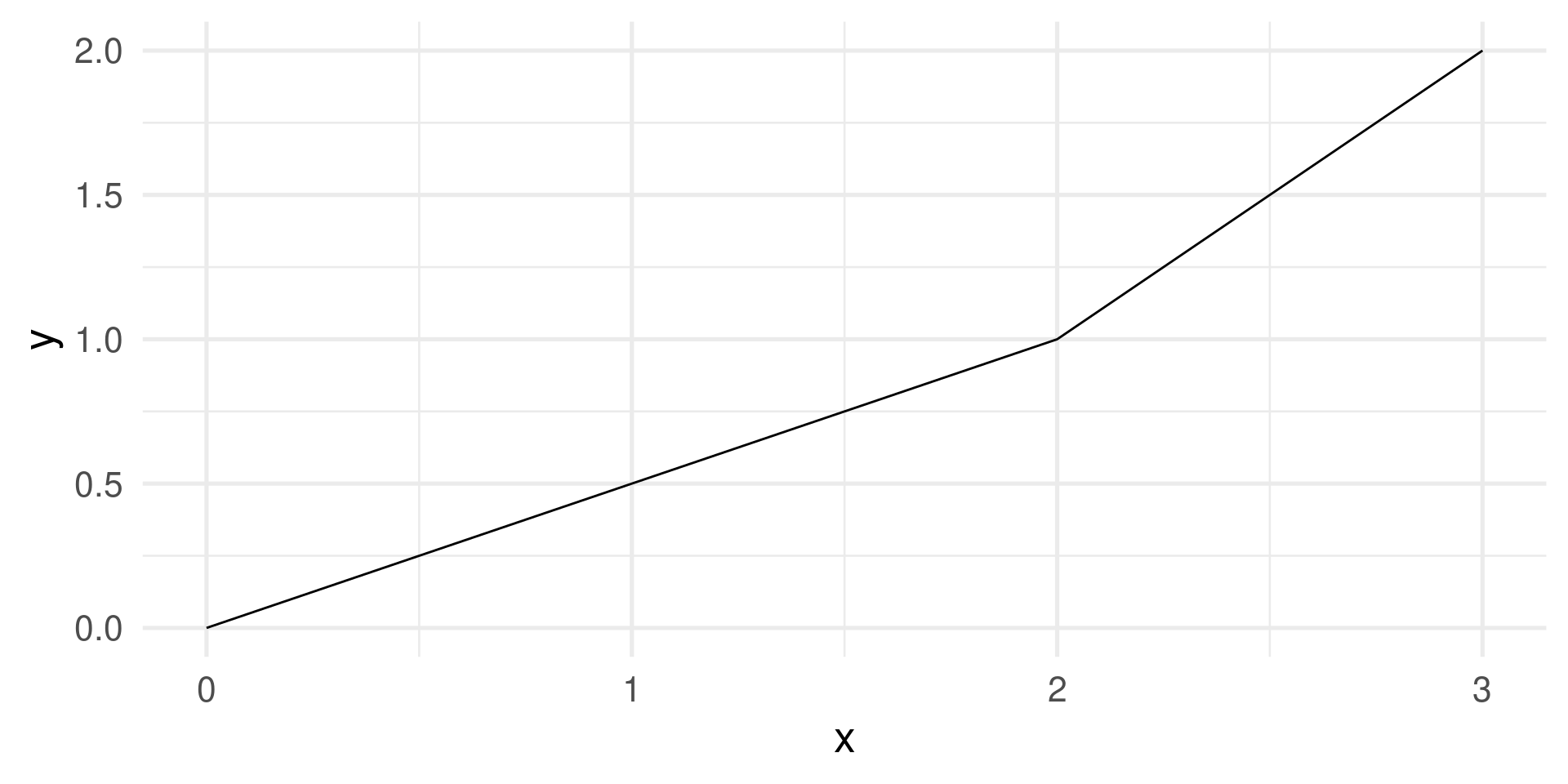
Example: A piece-wise defined function

piecewise <- function(x) {
  if (x < 2) {
    0.5 * x
  } else {
    x - 1
  }
}

piecewise(1)

[1] 0.5

piecewise(2)

[1] 1

piecewise(3)

[1] 2

Problem: piecewise is not vectorized. piecewise(c(1,2,3)) does not work.

Vectorized operations with map

• map functions apply a function to each element of a vector.¹
• map(.x, .f, ...) applies the function .f to each element of the vector of .x and returns a list.
• map_dbl returns a double vector (other variants exist)

map(c(1,2,3), piecewise) 

[[1]]
[1] 0.5

[[2]]
[1] 1

[[3]]
[1] 2

map_dbl(c(1,2,3), piecewise) 

[1] 0.5 1.0 2.0

piecewise_vectorized <- 
 function(x) map_dbl(x, piecewise) 

piecewise_vectorized(seq(0,3,by = 0.5))

[1] 0.00 0.25 0.50 0.75 1.00 1.50 2.00

tibble(x = seq(0,3,by = 0.5)) |> 
  mutate(y = piecewise_vectorized(x)) |> 
  ggplot(aes(x,y)) + geom_line() + theme_minimal(base_size = 20)

1. In tidyverse they are provided in the package purrr

map and reduce

Instead of a list or a vector reduce returns a single value.
To that end it needs a function with two arguments. It applies it to the first two elements of the vector, then to the result and the third element, then the result and the fourth element, and so on.

1:10 |> reduce(\(x,y) x + y)

[1] 55

Note: \(x) is a short way to write an anonymous function as function(x).

Example: Reading multiple files

Instead of

a <-read_csv("a.csv")
b <-read_csv("b.csv")
c <-read_csv("c.csv")
d <-read_csv("d.csv")
e <-read_csv("e.csv")
f <-read_csv("f.csv")
g <-read_csv("g.csv")

bind_rows(a,b,c,d,e,f,g)

Write

letter[1:7] |> 
 map(\(x) read_csv(paste0(x,".csv"))) |> 
 reduce(bind_rows)

Function programming: Take away

• Functions are the most important building blocks of programming.
• Functions can and often should be vectorized.
• Vectorized functions are the basis for plotting and transformation.
• map functions are powerful tools for iterative tasks!
  Expect to not get the idea first but to love them later.

Descriptive Statistics

Descriptive vs. Inferential Statistics

• The process of using and analyzing summary statistics
  • Solely concerned with properties of the observed data.
• Distinct from inferential statistics:
  • Inference of properties of an underlying distribution given sampled observations from a larger population.

Summary Statistics are used to summarize a set of observations to communicate the largest amount of information as simple as possible.

Summary statistics

Univariate (for one variable)

• Measures of location, or central tendency
• Measures of statistical dispersion
• Measure of the shape of the distribution like skewness or kurtosis

Bivariate (for two variables)

• Measures of statistical dependence or correlation

Measures of central tendency

Measures of central tendency

Goal: For a sequence of numerical observations \(x_1,\dots,x_n\) we want to measure

• the “typical” value.
• a value summarizing the location of values on the numerical axis.

Three different ways:

1. Arithmetic mean (also mean, average): Sum of the all observations divided by the number of observations \(\frac{1}{n}\sum_{i=1}^n x_i\)
2. Median: Assume \(x_1 \leq x_2 \leq\dots\leq x_n\). Then the median is middlemost values in the sequence \(x_\frac{n+1}{2}\) when \(n\) odd. For \(n\) even there are two middlemost values and the median is \(\frac{x_\frac{n}{2} + x_\frac{n+1}{2}}{2}\)
3. Mode: The value that appears most often in the sequence.

Philosophy of aggregation

• The mean represents total value per value.
  Example: per capita income in a town is the total income per individual
• The median represents the value such that half of the values are lower and higher.
  In a democracy where each value is represented by one voter preferring it, the median is the value which is unbeatable by an absolute majority. Half of the people prefer higher the other half lower values. (Median voter model)
• The mode represents the most common value.
  In a democracy, the mode represents the winner of a plurality vote where each value runs as a candidate and the winner is the one with the most votes.

Mean, Median, Mode properties

Do they deliver one unambiguous answer for any sequence?

Mean and median, yes.
The mode has no rules for a tie.

Can they by generalized to variables with ordered or even unordered categories?

Mean: No.
Median: For ordered categories (except when even number and the two middlemost are not the same) Mode: For any categorical variable.

Is the measure always also in the data sequence?

Mean: No.
Median: Yes, for sequences of odd length.
Mode: Yes.

Generalized means¹

For \(x_1, \dots, x_n > 0\) and \(p\in \mathbb{R}_{\neq 0}\) the generalized mean is

\[M_p(x_1, \dots, x_n) = (\frac{1}{n}\sum_{i=1}^n x_i^p)^\frac{1}{p}\]

For \(p = 0\) it is \(M_0(x_1, \dots, x_n) = (\prod_{i=1}^n x_i)^\frac{1}{n}\).

\(M_1\) is the arithmetic mean. \(M_0\) is called the geometric mean. \(M_{-1}\) the harmonic mean.

Note: Generalized means are often only reasonable when all values are positive \(x_i > 0\).

\(M_0\) can also be expressed as the exponential (\(\exp(x) = e^x\)) of the mean of the the \(\log\)’s of the \(x_i\)’s: \(\exp(\log((\prod_{i=1}^n x_i)^\frac{1}{n})) = \exp(\frac{1}{n}\sum_{i=1}^n\log(x_i))\).

1. Also called power mean or \(p\)-mean.

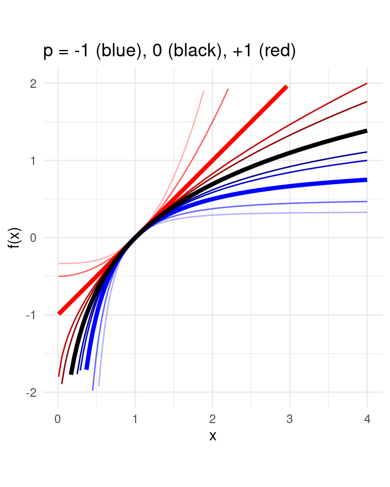
Box-Cox transformation function¹

For \(p \in \mathbb{R}\): \(f(x) = \begin{cases}\frac{x^p - 1}{p} & \text{for $p\neq 0$} \\ \log(x) & \text{for $p= 0$}\end{cases}\)

The \(p\)-mean is

\[M_p(x) = f^{-1}(\frac{1}{n}\sum_{i=1}^n f(x_i))\]

with \(x = [x_1, \dots, x_n]\). \(f^{-1}\) is the inverse² of \(f\).

1. Also a common transformation to pre-process data to make it closer to a normal distribution.

2. That means \(f^-1(f(x)) = x =f(f^-1(x))\).

Measures of central tendency and the Wisdom of the Crowd

Application: The Wisdom of the Crowd

• The collective opinion of a diverse group of independent individuals rather than that of a single expert.
• The classical wisdom-of-the-crowds finding is about point estimation of a continuous quantity.
• Popularized by James Surowiecki (2004).
• The opening anecdote is about Francis Galton’s¹ surprise in 1907 that the crowd at a county fair accurately guessed the weight of an ox’s meat when their individual guesses were averaged.

1. Galton (1822-1911) was a half-cousin to Charles Darwin and one of the founding fathers of statistics. He also was a scientific racist, see https://twitter.com/kareem_carr/status/1575506343401775104?s=20&t=8T5TzrayAWNShmOSzJgCJQ..

Galton’s data¹

What is the weight of the meat of this ox?

library(readxl)
galton <- read_excel("data/galton_data.xlsx")
galton |> ggplot(aes(Estimate)) + geom_histogram(binwidth = 5) + geom_vline(xintercept = 1198, color = "green") + 
 geom_vline(xintercept = mean(galton$Estimate), color = "red") + geom_vline(xintercept = median(galton$Estimate), color = "blue") + geom_vline(xintercept = Mode(galton$Estimate), color = "purple")

787 estimates, true value 1198, mean 1196.7, median 1208, mode 1218

1. Kenneth Wallis dug out the data from Galton’s notebook and put it here https://warwick.ac.uk/fac/soc/economics/staff/kfwallis/publications/galton_data.xlsx

Viertelfest Bremen 2008¹

How many lots will be sold by the end of the festival?

viertel <- read_csv("data/Viertelfest.csv")
viertel |> ggplot(aes(`Schätzung`)) + geom_histogram() + geom_vline(xintercept = 10788, color = "green") + 
 geom_vline(xintercept = mean(viertel$Schätzung), color = "red") + geom_vline(xintercept = median(viertel$Schätzung), color = "blue") + geom_vline(xintercept = Mode(viertel$Schätzung), color = "purple")

1226 estimates, the maximal value is 29530000!
We should filter out the highest values for the histogram…

1. Data collected as additional guessing game at the Lottery “Haste mal ’nen Euro?”, data provided by Jan Lorenz https://docs.google.com/spreadsheets/d/1HiYhUrYrsbeybJ10mwsae_hQCawZlUQFOOZzcugXzgA/edit#gid=0

Viertelfest Bremen 2008

How many lots will be sold by the end of the festival?

viertel <- read_csv("data/Viertelfest.csv")
viertel |> filter(Schätzung<100000) |> ggplot(aes(`Schätzung`)) + geom_histogram(binwidth = 500) + geom_vline(xintercept = 10788, color = "green") + 
 geom_vline(xintercept = mean(viertel$Schätzung), color = "red") + geom_vline(xintercept = median(viertel$Schätzung), color = "blue") + geom_vline(xintercept = Mode(viertel$Schätzung), color = "purple") + geom_vline(xintercept = exp(mean(log(viertel$Schätzung))), color = "orange")

1226 estimates, true value 10788, mean 53163.9, median 9843, mode 10000,
geometric mean 10510.1

\(\log_{10}\) transformation Viertelfest

viertel |> mutate(log10Est = log10(Schätzung)) |> ggplot(aes(log10Est)) + geom_histogram(binwidth = 0.05) + geom_vline(xintercept = log10(10788), color = "green") + 
 geom_vline(xintercept = log10(mean(viertel$Schätzung)), color = "red") + geom_vline(xintercept = log10(median(viertel$Schätzung)), color = "blue") + geom_vline(xintercept = log10(Mode(viertel$Schätzung)), color = "purple") + geom_vline(xintercept = mean(log10(viertel$Schätzung)), color = "orange")

1226 estimates, true value 10788, mean 53163.9, median 9843, mode 10000,
geometric mean 10510.1

Wisdom of the crowd insights

• In Galton’s sample the different measures do not make a big difference
• In the Viertelfest data the arithmetic mean performs very bad!
• The mean is vulnerable to extreme values.
  Quoting Galton on the mean as a democratic aggregation function:
  “The mean gives voting power to the cranks in proportion to their crankiness.”
• The mode tends to be on focal values as round numbers (10,000). In Galton’s data this is not so pronounced beause estimators used several units which Galton had to convert.
• How to choose a measure to aggregate the wisdom?
  • By the nature of the estimate problem? Is the scale mostly clear? (Are we in the hundreds, thousands, ten thousands, …)
  • By the nature of the distribution?
  • There is no real insurance against a systematic bias in the population.

Measures of dispersion

Measures of dispersion¹

Goal: We want to measure

• How spread out values are around the central tendency.
• How stretched or squeezed is the distribution?

Variance is the mean of the squared deviation from the mean: \(\text{Var}(x) = \frac{1}{n}\sum_{i=1}^n(x_i - \mu)^2\) where \(\mu\) (mu) is the mean.

Standard deviation is the square root of the variance \(\text{SD}(x) = \sqrt{\text{Var}(x)}\).

The standard deviation is often denoted \(\sigma\) (sigma) and the variance \(\sigma^2\).

Mean absolute deviation (MAD) is the mean of the absolute deviation from the mean: \(\text{MAD}(x) = \frac{1}{n}\sum_{i=1}^n|x_i - \mu|\).

Range is the difference of the maximal and the minimal value \(\max(x) - \min(x)\).

1. Also called variability, scatter, or spread.

Examples of measures of dispersion

var(galton$Estimate)

[1] 5415.013

sd(galton$Estimate)

[1] 73.58677

mad(galton$Estimate)

[1] 51.891

range(galton$Estimate)

[1]  896 1516

diff(range(galton$Estimate))

[1] 620

var(viertel$Schätzung)

[1] 719774887849

sd(viertel$Schätzung)

[1] 848395.5

mad(viertel$Schätzung)

[1] 8771.803

range(viertel$Schätzung)

[1]      120 29530000

diff(range(viertel$Schätzung))

[1] 29529880

Variance (and standard deviation) in statistics is usually computed with \(\frac{1}{n-1}\) instead of \(\frac{1}{n}\) to provide an unbiased estimator of the potentially underlying population variance. We omit more detail here.

Standardization

Variables are standardized by subtracting their mean and then dividing by their standard deviations.

A value from a standardized variable is called a standard score or z-score.

\(z_i = \frac{x_i - \mu}{\sigma}\)

where \(\mu\) is the mean and \(\sigma\) the standard deviation of the vector \(x\).

• This is a shift-scale transformation. We shift by the mean and scale by the standard deviation.
• A standard score \(z_i\) shows how mean standard deviations \(x_i\) is away from the mean of \(x\).

Achievements and next steps

• We have learned about the data science process
• You made essential steps in data visualization and data wrangling with New York City Flights in the Homework
• You can write and render reproducible reports
• We had some math refreshment
• We learned some data science data and programming concepts in R and in Python. Reconsider them in later homework!

Next steps coming (you will receive individual repositories for this):

• Homework mimicking data science projects
• Some exploratory data analysis in a sandbox
• Thinking about your own data science project (in groups of 2-3)